Three important components in solving NLA problems Development and analysis of numerical algorithms ●Perturbation theory ●Software Gene Golub/History of Numerical Linear Algebra
Three important components in solving NLA problems • Development and analysis of numerical algorithms • Perturbation theory • Software Gene Golub / History of Numerical Linear Algebra 5
A Fundamental Problem Problem:Suppose Ax=b+r, where A is an m x n matrix,and b is a given vector. Goal:Determine r such that rll min. Gene Golub/History of Numerical Linear Algebra 6
A Fundamental Problem Problem: Suppose Ax = b + r, where A is an m × n matrix, and b is a given vector. Goal: Determine r such that krk = min . Gene Golub / History of Numerical Linear Algebra 6
Important Parameters The relationship between m and n: overdetermined vs.'square'vs.underdetermined Uniqueness of solution The rank of the matrix A(difficult to handle if a small perturbation in A will change rank) 。Choice of norm ·Structure of A: -Sparsity Specialized matrices such as Hankel or Toeplitz Origin of problem:ideally,can make use of this in developing an algorithm. Gene Golub/History of Numerical Linear Algebra
Important Parameters • The relationship between m and n: – overdetermined vs. ‘square’ vs. underdetermined – Uniqueness of solution • The rank of the matrix A (difficult to handle if a small perturbation in A will change rank) • Choice of norm • Structure of A: – Sparsity – Specialized matrices such as Hankel or Toeplitz • Origin of problem: ideally, can make use of this in developing an algorithm. Gene Golub / History of Numerical Linear Algebra 7
Some Perturbation Theory Given Ax=6. and the perturbed system (A+△A)y=b+6, it can be shown that if N△AL≤e, deltal≤e, IA‖ b then lz-<2E·(A), Iz≤1-p where p=△A·IA-1‖=I△A‖·(A)/A‖<1, and (A)=‖A‖·‖A-1 Gene Golub/History of Numerical Linear Algebra 8
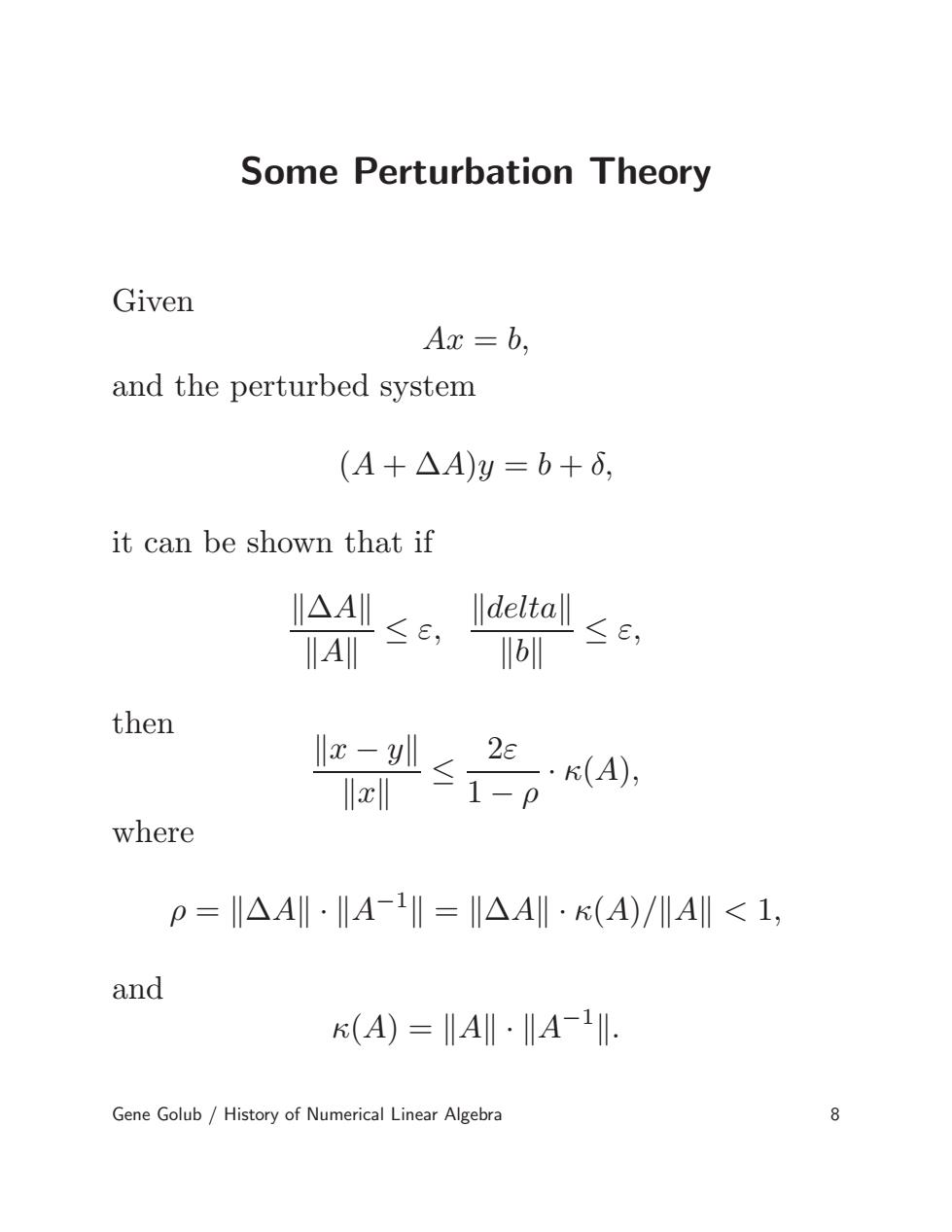
Some Perturbation Theory Given Ax = b, and the perturbed system (A + ∆A)y = b + δ, it can be shown that if k∆Ak kAk ≤ ε, kdeltak kbk ≤ ε, then kx − yk kxk ≤ 2ε 1 − ρ · κ(A), where ρ = k∆Ak · kA −1 k = k∆Ak · κ(A)/kAk < 1, and κ(A) = kAk · kA −1 k. Gene Golub / History of Numerical Linear Algebra 8
The Condition Number The quantity (A)=‖A‖·‖A-1‖ is called the condition number of A(or the condition number of the linear system). Note: even if s is small,a large k can be destructive a special relationship between A and 6 may further determine the conditioning of the problem A detailed theory of condition numbers: John Rice,1966. Gene Golub/History of Numerical Linear Algebra
The Condition Number The quantity κ(A) = kAk · kA −1 k is called the condition number of A (or the condition number of the linear system). Note: • even if ε is small, a large κ can be destructive • a special relationship between A and b may further determine the conditioning of the problem A detailed theory of condition numbers: John Rice, 1966. Gene Golub / History of Numerical Linear Algebra 9