上海交通大学：《复杂系统动力学计算机辅助分析》课程教学资源_Chapter 6_Char6.3 Equations of motion of constrained planar

6.3.3 Mixed differential-algebraic equations of motion There exists an m vectorA of Lagrange Multiplier such that δq(Mi-2+p,2)=0 for arbitraryδq Therefore,the coefficient of g must be zero,yielding the Lagrange multiplier form of equations Mi+D,2=24 Recall the velocity and acceleration equations 中1=-更，=v,中，i=-(Φ，)，i-2Φ9i-D1=Y Mixed differential-algebraic equations of motion 2-9

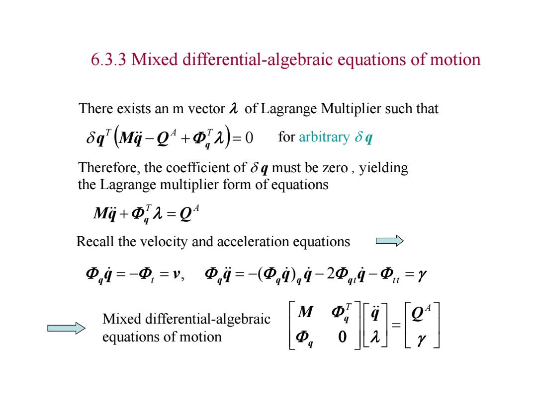
6.3.3 Mixed differential-algebraic equations of motion There exists an m vector l of Lagrange Multiplier such that    l  0 T A T Q q  q Mq for arbitrary  q Therefore, the coefficient of  q must be zero , yielding the Lagrange multiplier form of equations T A Mq q l  Q Recall the velocity and acceleration equations              t t tt q v q q q q q q q q q  ,  ( )  2                   l   T A M q Q q q   Mixed differential-algebraic equations of motion

Two formulations for solving dynamic problem δg(M-Q4）=0 0 Compressive formulation Expansion formulation q=Dq 6q(Mi-2+Φ，2=0 g Independent coordinate vector →Mi-2+Φ，2=0 →δ7(D'MDi-D2)=0 D'MDG-D'Q →&8-e] ·Easy for solution Expensive for calculation No constraint force results Constraint force results ·For special case ·For general case

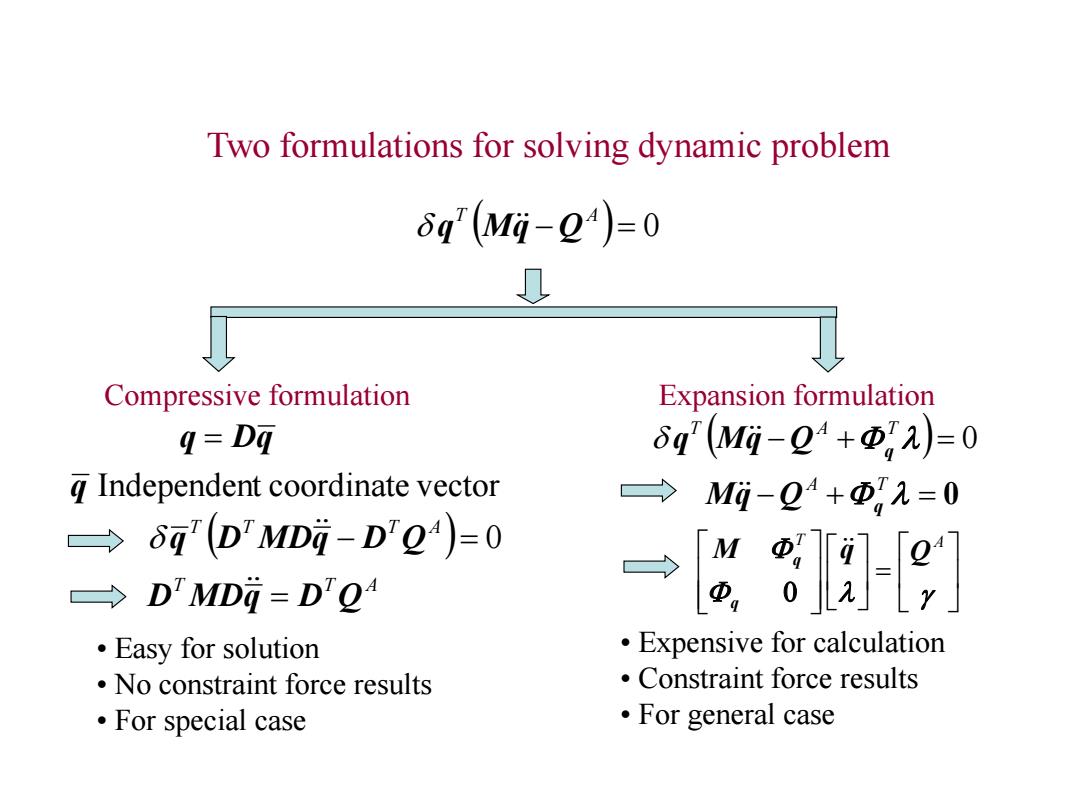
Two formulations for solving dynamic problem    0 T A  q Mq Q q  Dq    0 T T T A  q D MDq D Q q Independent coordinate vector T T A D MDq   D Q • Easy for solution • No constraint force results • For special case Compressive formulation Expansion formulation    l  0 T A T Q q  q Mq  l  0 A T Q q Mq                  l   T A M q Q q q   • Expensive for calculation • Constraint force results • For general case

Constraint dynamic existence theorem Condition (I)Φ，has full row rank (2)dMod>0 for any nonzero virtual velocity that is consistent with the constraint Result For allδi≠0 is nonsingular ,A are uniquely determined Failure (1)Singular configurafiares (2)System with redundant joints (3)M is not positive,that is,some of the diagonal elements vanish

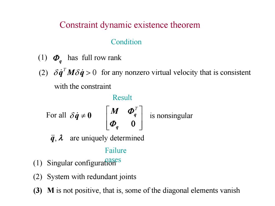
Constraint dynamic existence theorem  q (1) has full row rank Condition For all  q  0 is nonsingular      q M q   T q, l are uniquely determined (1) Singular configuration (2) System with redundant joints (3) M is not positive, that is, some of the diagonal elements vanish  q M q  0 T (2) for any nonzero virtual velocity that is consistent with the constraint Result Failure cases

Initial position condition System constraint equations involve both kinematic and driving constraint of the form g-08 Initial position conditions are defined in the form ow-- Which is required that (1)The number of the equations be equal to the number of system degrees of freedom (2)(g(t),t)=0 must be independent to uniquely determine g(to)

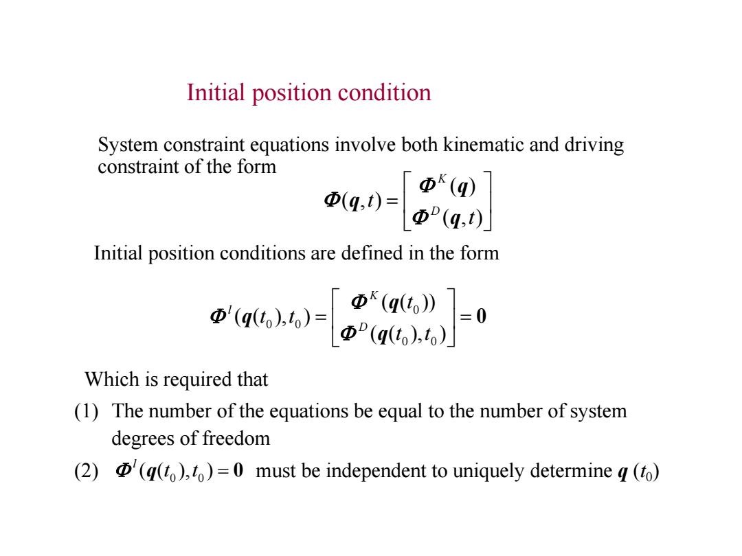
Initial position condition        ( , ) ( ) ( , ) t t D K q q q    Initial position conditions are defined in the form   0       ( ( ), ) ( ( )) ( ( ), ) 0 0 0 0 0 t t t t t D K l q q q    Which is required that (1) The number of the equations be equal to the number of system degrees of freedom (2) must be independent to uniquely determine q (t0 ( ( ), )  0 ) 0 0 t t l  q System constraint equations involve both kinematic and driving constraint of the form

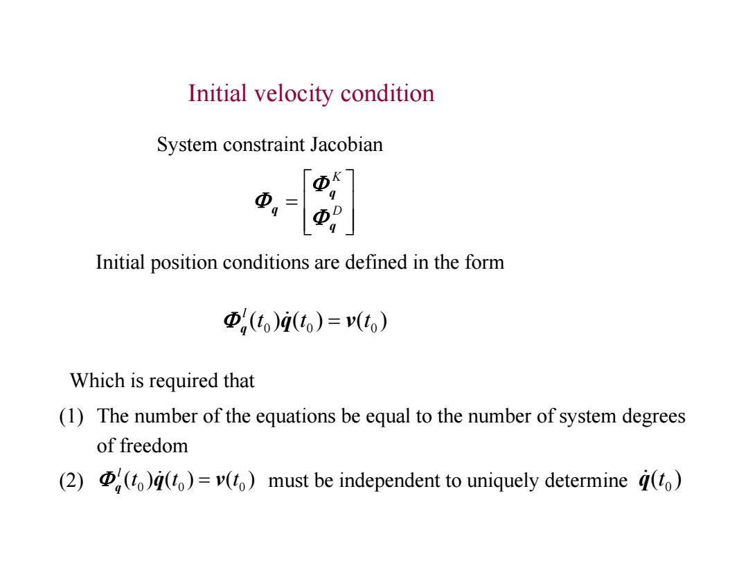
Initial velocity condition System constraint Jacobian Initial position conditions are defined in the form Φ，(to)i(t)=v(to) Which is required that (1)The number of the equations be equal to the number of system degrees of freedom (2)()()=v(t)must be independent to uniquely determine a(t)

Which is required that (1) The number of the equations be equal to the number of system degrees of freedom (2) (t0 ) (t0 ) (t0 ) must be independent to uniquely determine l q v  q   ( )0 q t Initial velocity condition      D K q q q    Initial position conditions are defined in the form ( ) ( ) ( ) 0 0 0 t t t l q v  q   System constraint Jacobian