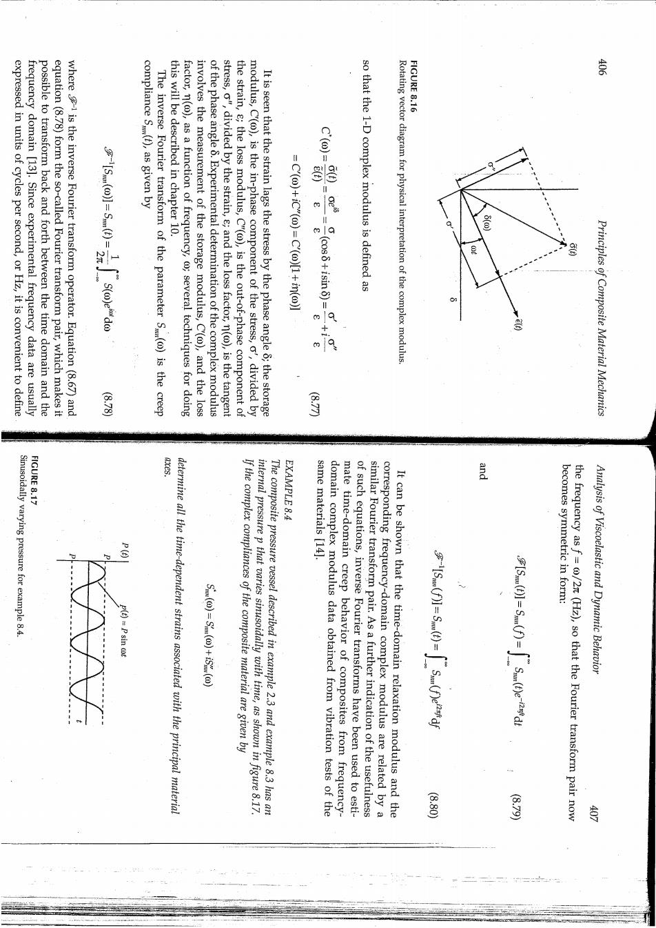
FIGURE 8.16 expressed in units of cycles per second,or Hz,it is convenient to define frequency domain [13].Since experimental frequency data are usually possible to transform back and forth between the time domain and the equation(8.78)form the so-called Fourier transform pair,which makes it where91 is the inverse Fourier transform operator.Equation(8.67)and compliance S(t),as given by The inverse Fourier transform of the parameter S()is the creep this will be described in chapter 10. factor,n(o),as a function of frequency,o;several techniques for doing involves the measurement of the storage modulus,C(o),and the loss of the phase angle 8.Experimental determination of the complex modulus stress,o",divided by the strain,e;and the loss factor,n(),is the tangent the strain,e;the loss modulus,C"(),is the out-of-phase component of modulus,C(o),is the in-phase component of the stress,o',divided by It is seen that the strain lags the stress by the phase angle 8;the storage -Q⑧)+nB)1Q(B+3e二 (cos8+isin8)= so that the 1-D complex modulus is defined as Rotating vector diagram for physical interpretation of the complex modulus 9 Principles of Composite Material Mechanics 8.78 S77 FIGURE 8.17 axes. Sinusoidally varying pressure for example 8.4. EXAMPLE 8.4 same materials [14] P() p(t)=P sin ot determine all the time-dependent strains associated with the principal material ¥e)⑧+e) internal pressure p that varies sinusoidally with time,as shown in figure 8.17 If the complex compliances of the composite material are given by The composite pressure vessel described in example 2.3 and example 8.3 has an mate time-domain creep behavior of composites from frequency- domain complex modulus data obtained from vibration tests of the of such equations,inverse Fourier transforms have been used to esti- corresponding frequency-domain complex modulus are related by a similar Fourier transform pair.As a further indication of the usefulness It can be shown that the time-domain relaxation modulus and the becomes symmetric in form: the frequency as f=/2n(Hz),so that the Fourier transform pair now Analysis of Viscoelastic and Dynamic Behavior 6.50) 679

tions are and the variational methods of elastic analysis are beyond the scope of equations,the strain-displacement relations,the boundary conditions, solution to an elasticity problem.The correspondences in the equilibriun relationships,there are obviously other equations involved in a complete table 8.1 is only concerned with the correspondences in the stress-strain equations to get the corresponding linear viscoelastic solution.Although to a problem,we simply make the corresponding substitutions in the table is that if we have the necessary equations for a linear elastic solution stress-strain relationships is given in table 8.1.The implication of this A summary of the correspondences between elastic and viscoelastic detail by Schapery [1,17]and Christensen [6]. the viscoelastic analysis of anisotropic composites has been discussed in by Biot [16].The specific application of the correspondence principle to by Lee[151,whereas the application to anisotropic materials was proposed respondence principle for isotropic materials was apparently introduced ognition of an "Elastic-Viscoelastic Correspondence Principle."The cor- equations for elastic and viscoelastic analysis have led to the formal rec- the same as that for linear elastic materials.Such analogies between the form of the stress-strain relationships for linear viscoelastic materials is In the previous sections,we have seen a number of examples where the 8.2.5.Elastic-Viscoelastic Correspondence Principle [S()+iS()16.0Psin ct 0m0*+18-(/+56(01707-64-0+6:(0120.59 = E2(t)=Si2()G1(E)+S22(@)G2(t)+(O)G6(E) +m4+15:(09g:(0l7.0(a.1(0+63T0:120.57 The corresponding strains from equations(8.70)are 6(t)=1()=6.0p=6.0P sinct(MPa) :aP制。71-00.71-)分G2 1(t)=20.5p=20.5P sin (t(MPa) Solution.From example 2.3 and figure 8.17,the stresses along the 12 direc- Principles of Composite Material Mechanics where Input strains Input stresses Linear Elastic TABLE 8.1 epoxy composite are shown in figure 8.18 from ref.I181.From these resnlts of a similar analysis of the creep compliances S2()and S6()for a glass Generalized creep Linear Viscoelastic the time dependency of E(t)would be governed by Em(f)alone.The results that of the fiber,so the fiber modulus could be assumed to be elastic,and ther simplification possible.In most polymer matrix composites,the time dependency of the matrix material would be much more significant than The relative viscoelasticity of fiber and matrix materials may make fur- vm=matrix volume fraction v:=fiber volume fraction E(f)=relaxation modulus of isotropic matrix En(f)=longitudinal relaxation modulus of fiber E1(t)=longitudinal relaxation modulus of composite B电-Em+君r电ai a unidirectional composite can now be converted for viscoelastic relax- ation problems by rewriting equation(3.23)as example,the rule of mixtures for predicting the longitudinal modulus of converted for prediction of the corresponding viscoelastic properties.For is that analytical models for predicting elastic properties of composites at both the micromechanical and the macromechanical levels can be easily Constant stress creep One of the most important implications of the correspondence principle and Christensen [4,6]. this book,but detailed discussions of these are given by Schapery [1,17] Sinusoidal strain input Sinusoidal stress input Constant strain relaxation Generalized relaxation Material and Input 9 9 Stresses Analysis of Viscoelastic and Dynamic Behavior 器 Strains Elastic-Viscoelastic Correspondence in Stress-Strain Relationships Properties 8.81) 18.7 Equation
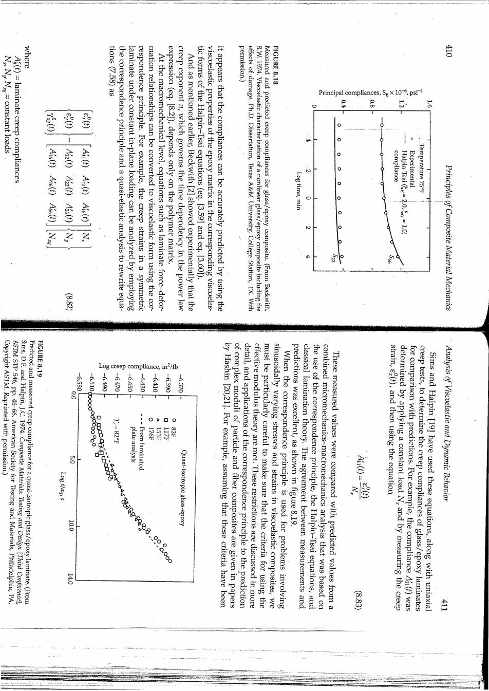
where NN,Ny=constant loads A(t)=laminate creep compliances tions (7.58)as permission.) FIGURE 8.18 Principal compliances,S106,psi-1 晋 墨 器 Aic(E)Az6(E)Ads(t) Ai()Ai2(t)Ai6(t) expression (eq.[8.21),depends only on the polymer matrix. compliance Log time,min Halpin-Tsai (=2.0,G=1.0) Experimental Temperature 75F o o 子 the correspondence principle and a quasi-elastic analysis to rewrite equa- laminate under constant in-plane loading can be analyzed by employing respondence principle.For example,the creep strains in a symmetric mation relationships can be converted to viscoelastic form using the cor- At the macromechanical level,equations such as laminate force-defor- creep exponent n,which governs the time dependency in the power law And as mentioned earlier,Beckwith [2]showed experimentally that the tic forms of the Halpin-Tsai equations (eq.[3.59]and eq.[3.601). viscoelastic properties of the epoxy matrix in the corresponding viscoelas- it appears that the compliances can be accurately predicted by using the effects of damage.Ph.D.Dissertation,Texas A&M University,College Station,TX.With S.W.1974.Viscoelastic characterization of a nonlinear glass/epoxy composite including the Measured and predicted creep compliances for glass/epoxy composite.(From Beckwith, e e Principles of Composite Material Mechanics Copyright ASTM.Reprinted with permission.) FIGURE 8.19 Log creep compliance, n2/Ib -6.530 -6.510 -6.490 -6.470 -6.450 6.430 6010 -6.390 -6.370 ASTM STP 546,pp.46-66.American Society for Testing and Materials,Philadelphia,PA. Sims,D.F.and Halpin,J.C.1974.Composite Materials:Testing and Design [Third Conferencel Predicted and measured creep compliance for a quasi-isotropic glass/epoxy laminate.(From plate analysis From laminated strain,e(t),and then using the equation Analysis of Viscoelastic and Dynamic Behavior Log tlan s Quasi-isotropic glass-epoxy predictions was excellent,as shown in figure 8.19. 100 00 by Hashin [20,211.For example,assuming that these criteria have been of complex moduli of particle and fiber composites are given in papers detail,and applications of the correspondence principle to the prediction must be particularly careful to make sure that the criteria for using the effective modulus theory are met.These restrictions are discussed in more sinusoidally varying stresses and strains in viscoelastic composites,we When the correspondence principle is used for problems involving classical lamination theory.The agreement between measurements and the use of the correspondence principle,the Halpin-Tsai equations,and combined micromechanics-macromechanics analysis that was based on These measured values were compared with predicted values from a determined by applying a constant load N,and by measuring the creep for comparison with predictions.For example,the compliance Ai(t)was creep tests,to determine the creep compliances of glass/epoxy laminates Sims and Halpin [19]have used these equations,along with uniaxial 140 B.83 兰
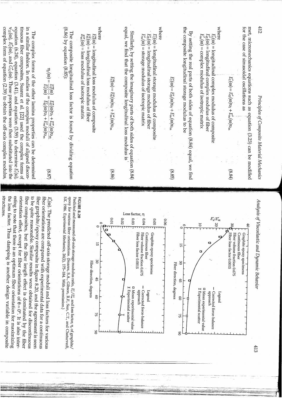
where where where 常 complex form of equation(2.39)to obtain the off-axis complex modulus, Vi2(),E2(),and Gi2().These properties were then substituted into the equation (6.24),equation (3.41),and equation(3.59)to determine Ei(), tinuous fiber composites,Suarez et al.[22]used the complex forms of in a similar fashion.In studies of the complex moduli of aligned discon- The complex forms of the other lamina properties can be determined (8.86)by equation (8.85): 主③ Em(@)=loss modulus of isotropic matrix E(@)=longitudinal loss modulus of fiber for the case of sinusoidal oscillations as E()v:+Em()vm The composite longitudinal loss factor is found by dividing equation E()=longitudinal loss modulus of composite 8-(82+=(8d equal,we find that the composite longitudinal loss modulus is Similarly,by setting the imaginary parts of both sides of equation(8.84) En (@)=storage modulus of isotropic matrix En(@)=longitudinal storage modulus of fiber Ei()=longitudinal storage modulus of composite the composite longitudinal storage modulus to be By setting the real parts of both sides of equation(8.84)equal,we find Em()=complex modulus of isotropic matrix En(@)=longitudinal complex modulus of fiber E()=longitudinal complex modulus of composite E()=En()vi+Em()vm met,micromechanics equations such as equation(3.23)can be modified Principles of Composite Material Mechanics 图 至 FIGURE 8.20 Loss factor,n 0.02 0.06 Ej/E the loss factor.Thus damping is another design variable in composite structures. esting to note that there is an optimum fiber orientation for maximizing orientation effect,except for fiber orientations of 0=0.It is also inter- 名 fiber composites,but the fiber length effect is dominated by the fiber to be quite reasonable.Similar results were obtained for discontinuous fiber graphite/epoxy composite in figure 8.20,and the agreement is seen fiber orientations are compared with experimental data for a continuous E().The predicted off-axis storage moduli and loss factors for various S.K.1986.Experimental Mechanics,26(2),175-184.With permission.) epoxy for various fiber orientations. Predicted and measured off-axis storage modulus ratio,EEand loss factor,of graphite/ 0 Fiber loss factor 0.0015 Fiber volume fraction 0.675 Continuous fiber Graphite epoxy specimens Fiber loss factor 0.0015 Fiber volume fraction 0.675 Continuous fiber Graphite epoxy specimens Analysis of Viscoelastic and Dynamic Behavior (Suarez,S.A.,Gibson,R.F,Sun,C.T.,and Chaturvedi Fiber direction,degrees Fiber direction,degrees g I Experimental scatter Mean experimental value approach Corrected force-balance Legend I Experimental scatter D Mean experimental value approach Corrected force-balance 请Le 会
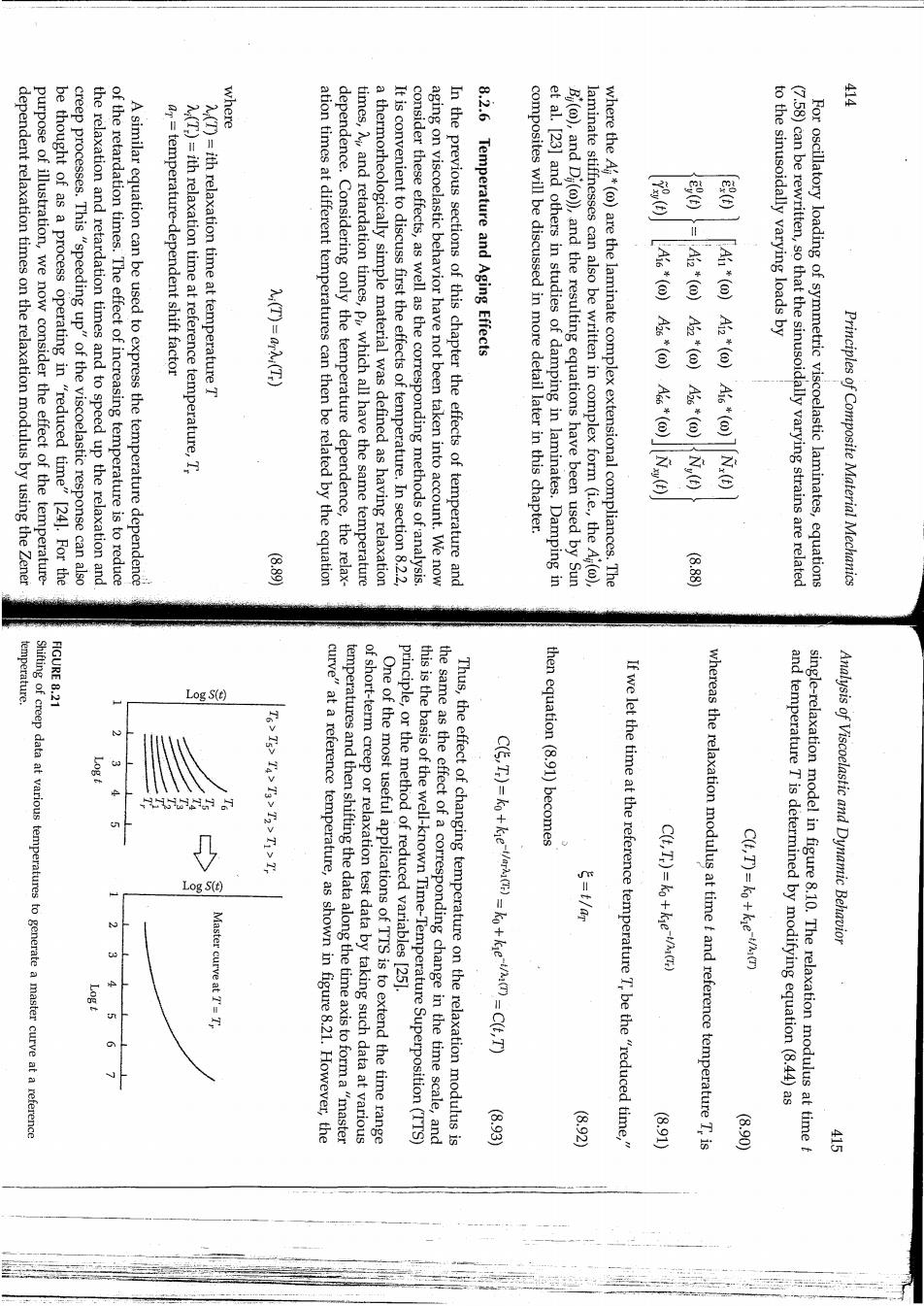
where dependent relaxation times on the relaxation modulus by using the Zener purpose of illustration,we now consider the effect of the temperature- be thought of as a process operating in "reduced time"[24].For the creep processes.This "speeding up"of the viscoelastic response can also the relaxation and retardation times and to speed up the relaxation and of the retardation times.The effect of increasing temperature is to reduce A similar equation can be used to express the temperature dependence ar=temperature-dependent shift factor A(T)=ith relaxation time at reference temperature,T; A(T)=ith relaxation time at temperature T ation times at different temperatures can then be related by the equation dependence.Considering only the temperature dependence,the relax- times,and retardation times,Pi which all have the same temperature a thermorheologically simple material was defined as having relaxation It is convenient to discuss first the effects of temperature.In section 8.2.2 consider these effects,as well as the corresponding methods of analysis aging on viscoelastic behavior have not been taken into account.We now In the previous sections of this chapter the effects of temperature and 8.2.6 Temperature and Aging Effects composites will be discussed in more detail later in this chapter. et al.[23]and others in studies of damping in laminates.Damping in B(),and Di()),and the resulting equations have been used by Sun laminate stiffnesses can also be written in complex form (i.e.,the Aj(o) where the A*()are the laminate complex extensional compliances.The 器 to the sinusoidally varying loads by 中国好国的国 (7.58)can be rewritten,so that the sinusoidally varying strains are related For oscillatory loading of symmetric viscoelastic laminates,equations Principles of Composite Material Mechanics 图 (8.88 emperature. FIGURE 8.21 Log S(t) Shifting of creep data at various temperatures to generate a master curve at a reference principle,or the method of reduced variables [25]. then equation(8.91)becomes Log S(t) C(t,Tr)=ko+ke-t/M(E) C(t,T)=ko+kie-t/a(r) Analysis of Viscoelastic and Dynamic Behavior 5 Master curve at T'=T, C(Tr)=ko+ke-t/arki()=ko+ke-ta()=C(t,T) 56 curve"at a reference temperature,as shown in figure 8.21.However,the temperatures and then shifting the data along the time axis to form a"master of short-term creep or relaxation test data by taking such data at various One of the most useful applications of TTS is to extend the time range this is the basis of the well-known Time-Temperature Superposition(TTS) the same as the effect of a corresponding change in the time scale,and Thus,the effect of changing temperature on the relaxation modulus is If we let the time at the reference temperatureTbe the"reduced time" whereas the relaxation modulus at time f and reference temperature T,is and temperature T is determined by modifying equation(8.44)as single-relaxation model in figure 8.10.The relaxation modulus at time t 图 (6.00