Example 6.1.The slope field for y'=(t-y)/2 over the rectangle R=(ty):05,0<4)is shown in the figure.The solution curves with the following initial values are shown: 1.For y(0)=1,the solution is v(t)=3e-42-2+t; 2.For y(0)=4,the solution is y(1)=6e42-2+t. 4.5 3.5
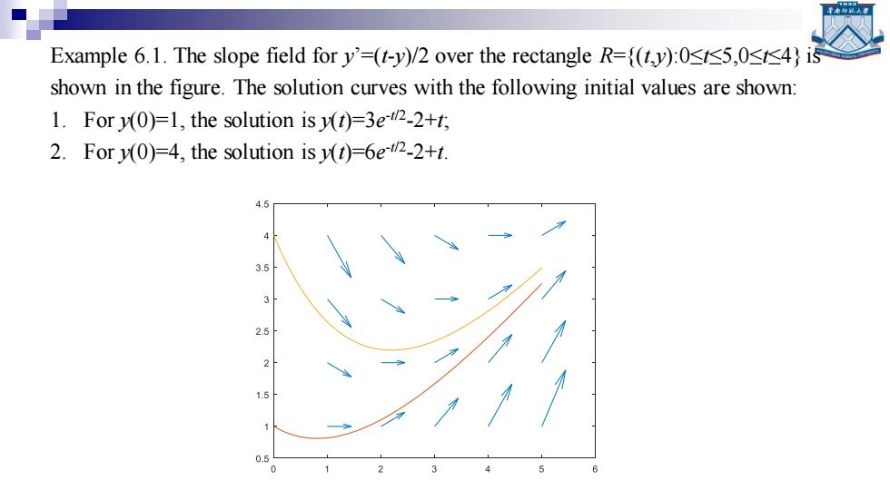
Example 6.1. The slope field for y’=(t-y)/2 over the rectangle R={(t,y):0≤t≤5,0≤t≤4} is shown in the figure. The solution curves with the following initial values are shown: 1. For y(0)=1, the solution is y(t)=3e -t/2 -2+t; 2. For y(0)=4, the solution is y(t)=6e -t/2 -2+t
Lipschitz condition ■Def.6.2.Given the rectangle R={(t,y):a≤b,c≤d,assume thatt,.y) is continuous on R.The function fis said to satisfy a Lipschitz condition in the variable y on R provided that a constant L>0 exists with the property that t,y)ft,y2Ll,whenever (t,y),(t,y2)ER.The constant L is called a Lipschitz constant for f. Thm.6.1.Suppose that f(t,y)is defined on the region R.If there exists a constant L>0 so that f(t,y)L for all (t,y)ER,then fsatisfies a Lipschitz condition in the variable y with Lipschitz constant L over the rectangle R
Lipschitz condition ◼
Existence and Uniqueness Thm.6.2.Assume that f(t,y)is continuous in a region R={(t,y): totb,csysd).If fsatisfies a Lipschitz condition on R in the variabley and (to,)ER,then the initial value problem in Def 6.1,y'=ft,y)with y(to)=yo,has a unique solution y=y(t)on some subinterval to<tto+. For the function ft,y)=(t-y)/2 in example 6.1,The partial derivative isf(t,y)=-1/2.Hence(t,y)1/2 and,according to Thm.6.1,the Lipschitz constant is L=1/2.Therefore,by Thm. 6.2 the I.V.P.has a unique solution
Existence and Uniqueness ◼

Euler's Method Not all initial value problems can be solved explicitly,and often it is impossible to find a formula for the solution t). For engineering and scientific purpose it is necessary to have methods for approximating the solution.If a solution with many significant digits is required,then more computing effort and a sophisticated algorithm must be used. The first approach,called Euler's method,serves to illustrate the concepts involved in the advanced methods.It has limited use because of the larger error that is accumulated as the process proceeds.However,it is important to study because the error analysis is easier to understand
Euler’s Method ◼ Not all initial value problems can be solved explicitly, and often it is impossible to find a formula for the solution y(t). ◼ For engineering and scientific purpose it is necessary to have methods for approximating the solution. If a solution with many significant digits is required, then more computing effort and a sophisticated algorithm must be used. ◼ The first approach, called Euler’s method, serves to illustrate the concepts involved in the advanced methods. It has limited use because of the larger error that is accumulated as the process proceeds. However, it is important to study because the error analysis is easier to understand

Euler's Approximation Let [a,b]be the interval over which we want to find the solution to the well-posed I.V.P.y'=ft)with y(a)=vo.For convenience we subdivide the interval [a,b]into M equal subintervals and select the mesh points a=b<h<b<.....<tv-<=b, 1=o+kh,for k=1,2....,M where h=b-a The value h is called the step size.We now proceed to solve approximately y'At,y)over [to,tul with y(to)=yo. (6.11) Assume that yt),y(t),and y(t)are continuous and use Taylor's theorem to expand y(t) about t=t.For each value t there exists a value cI that lies between to and t so that
Euler’s Approximation 0 1 2 1 0 , , for 1,2, , where . M M k a t t t t t b b a t t kh k M h M = = − − = + = = ◼ Let [a, b] be the interval over which we want to find the solution to the well-posed I.V.P. y’=f(t,y) with y(a)=y0 . For convenience we subdivide the interval [a, b] into M equal subintervals and select the mesh points The value h is called the step size. We now proceed to solve approximately y’=f(t, y) over [t0 , tM] with y(t0 )=y0 . Assume that y(t), y’(t), and y’’(t) are continuous and use Taylor’s theorem to expand y(t) about t=t0 . For each value t there exists a value c1 that lies between t0 and t so that (6.11)