The Grand Checklist Normality:plot histogram of the residuals. Standardized residuals Heteroscedasticity: plot residuals with each x variables,transform if necessary, Box-Cox transformations. .Autocorrelation:“time series plot” Multicollinearity:compute correlations of the x variables, do signs of coefficients agree with intuition? Principal components Missing Values DATA Copyright 2019 by Xiaoyu Li
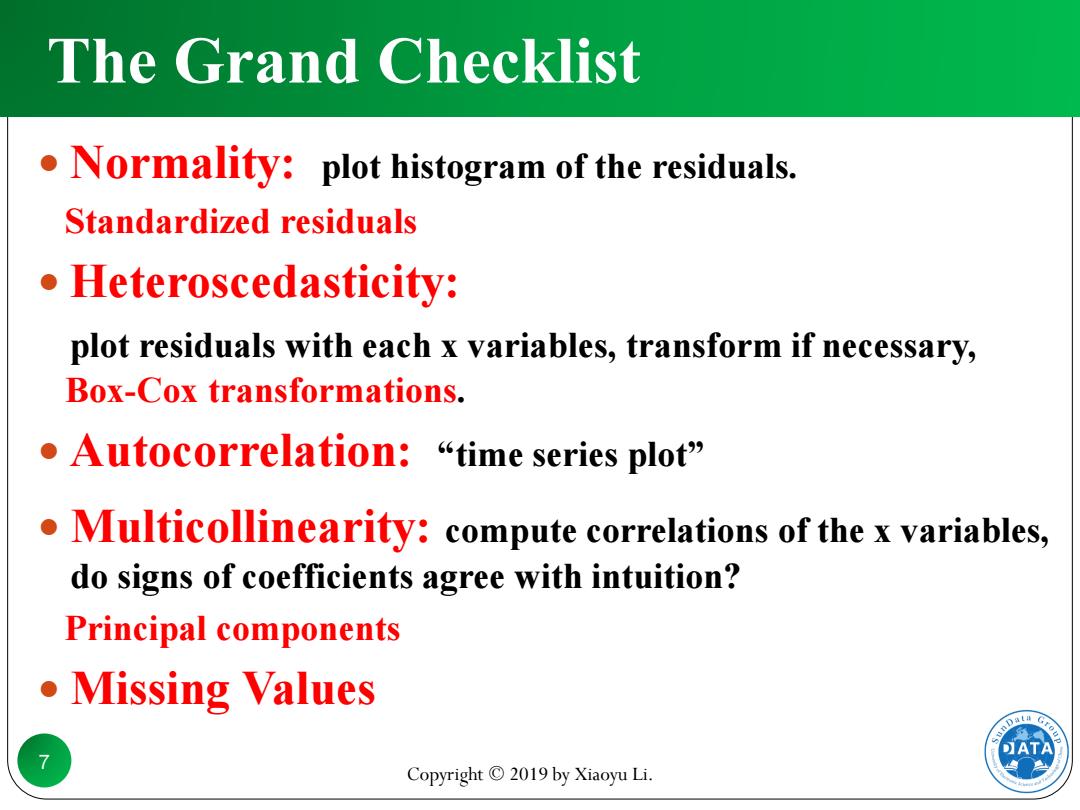
Copyright © 2019 by Xiaoyu Li. 7 The Grand Checklist Normality: plot histogram of the residuals. Standardized residuals Heteroscedasticity: plot residuals with each x variables, transform if necessary, Box-Cox transformations. Autocorrelation: “time series plot” Multicollinearity: compute correlations of the x variables, do signs of coefficients agree with intuition? Principal components Missing Values

Group Today Topic encead Logistic Regression 8 Copyright 2019 by Xiaoyu Li
Today Topic Copyright © 2019 by Xiaoyu Li. 8 Logistic Regression
Logistic Regression Introduction Developed by statistician David Cox in 1958; Extends the ideas of multiple linear regression to the situation where the dependent variable is binary; Further,a regression model where the dependent variable (DV)is categorical; An alternative to Fisher's 1936 classification method; .Independent variablesxx2...x categorical or continuous variables or a mixture of these two types. ATA 9 Copyright 2019 by Xiaoyu Li
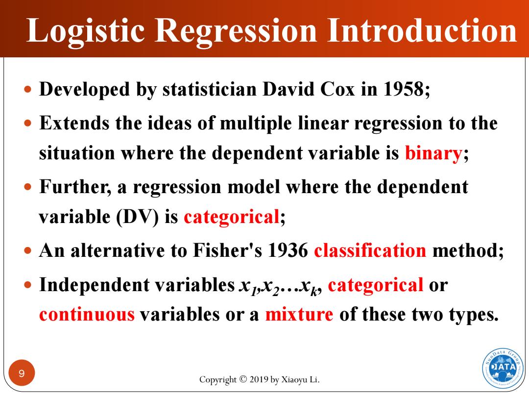
Copyright © 2019 by Xiaoyu Li. 9 Logistic Regression Introduction Developed by statistician David Cox in 1958; Extends the ideas of multiple linear regression to the situation where the dependent variable is binary; Further, a regression model where the dependent variable (DV) is categorical; An alternative to Fisher's 1936 classification method; Independent variables x1 ,x2…xk , categorical or continuous variables or a mixture of these two types
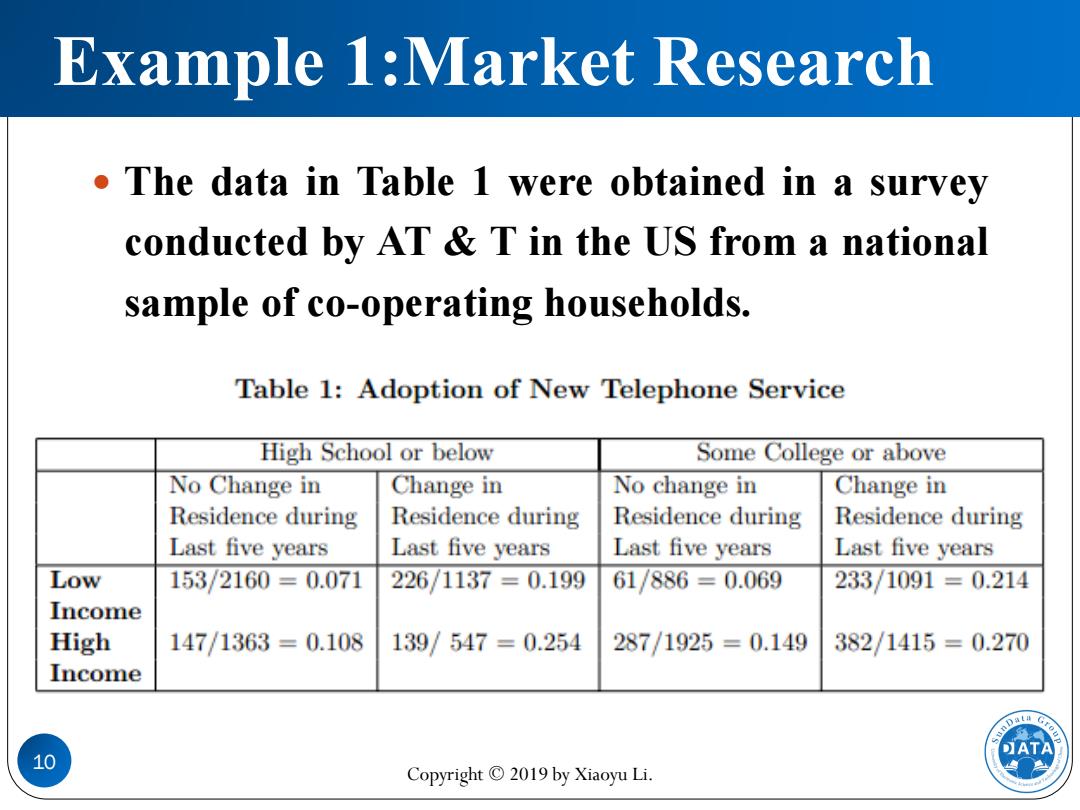
Example 1:Market Research The data in Table 1 were obtained in a survey conducted by AT T in the US from a national sample of co-operating households. Table 1:Adoption of New Telephone Service High School or below Some College or above No Change in Change in No change in Change in Residence during Residence during Residence during Residence during Last five years Last five years Last five years Last five years Low 153/2160=0.071 226/1137=0.199 61/886=0.069 233/1091=0.214 Income High 147/1363=0.108 139/547=0.254 287/1925=0.149 382/1415=0.270 Income ATA 10 Copyright 2019 by Xiaoyu Li
Copyright © 2019 by Xiaoyu Li. 10 Example 1:Market Research The data in Table 1 were obtained in a survey conducted by AT & T in the US from a national sample of co-operating households
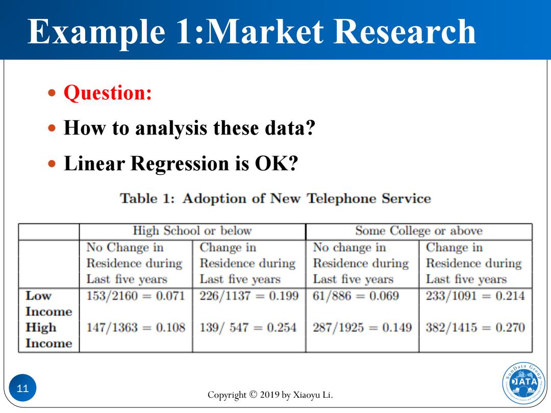
Example 1:Market Research Question: How to analysis these data? Linear Regression is OK? Table 1:Adoption of New Telephone Service High School or below Some College or above No Change in Change in No change in Change in Residence during Residence during Residence during Residence during Last five years Last five years Last five years Last five years Low 153/2160=0.071 226/1137=0.199 61/886=0.069 233/1091=0.214 Income High 147/1363=0.108 139/547=0.254 287/1925=0.149 382/1415=0.270 Income ATA 11 Copyright 2019 by Xiaoyu Li
Copyright © 2019 by Xiaoyu Li. 11 Example 1:Market Research Question: How to analysis these data? Linear Regression is OK?