Rules for Obtaining the Quartile values 。 If the resulting positioning point is an integer number,then the particular numerical observation corresponding to that positioning point is chosen for the quartile. Rule 2:If the resulting positioning point is halfway between two integers(2.5,3.5,etc),then the quartile is equal to the average of the corresponding ranked values (observations). Rule 3:If the resulting positioning point is neither an integer nor a fractional half,you round the result and select that ranked value. Statistics for Mar agers Using Microsoft Excel Chap 3-16
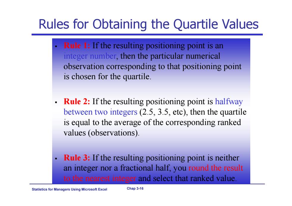
Statistics for Managers Using Microsoft Excel Chap 3-16 Rules for Obtaining the Quartile Values Rule 1: If the resulting positioning point is an integer number, then the particular numerical observation corresponding to that positioning point is chosen for the quartile. Rule 2: If the resulting positioning point is halfway between two integers (2.5, 3.5, etc), then the quartile is equal to the average of the corresponding ranked values (observations). Rule 3: If the resulting positioning point is neither an integer nor a fractional half, you round the result to the nearest integer and select that ranked value
Quartiles:Locating the First Quartile Example:Find the first quartile and third quartile Sample Data in Ordered Array:11 12 13 1616 17 18 21 22 First,note that n=9 Q=is in the (9+1)/4=2.5 ranked value of the ranked data,so use the value half way between the 2nd and 3rd ranked values,so Q=12.5 Q3 is in the 3*(9+1)/4=7.5 ranked value of the ranked data,so use the value half way between the 7th and 8th ranked values,so Q1=19.5 Q and Q,are measures of non-central location SPSS Q,=median,a measure of central tendency Statistics Microsoft Excel Chap 3-17
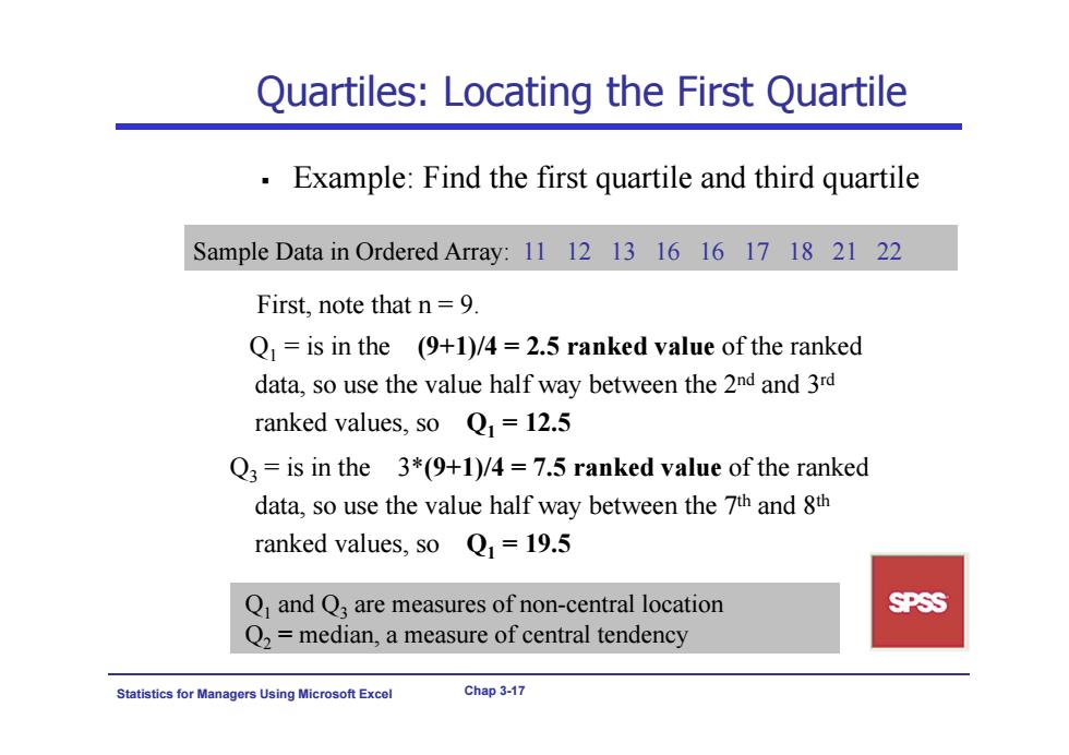
Statistics for Managers Using Microsoft Excel Chap 3-17 Quartiles: Locating the First Quartile Example: Find the first quartile and third quartile Sample Data in Ordered Array: 11 12 13 16 16 17 18 21 22 First, note that n = 9. Q1 = is in the (9+1)/4 = 2.5 ranked value of the ranked data, so use the value half way between the 2nd and 3rd ranked values, so Q1 = 12.5 Q3 = is in the 3*(9+1)/4 = 7.5 ranked value of the ranked data, so use the value half way between the 7th and 8th ranked values, so Q1 = 19.5 Q1 and Q3 are measures of non-central location Q2 = median, a measure of central tendency

Geometric Mean Useful in the measure of rate of change of a variable over time The geometric mean is the nt root of the product of n values. xG=(X,×X2×xXn)” Geometric mean rate of return Measures the status of an investment over time R。=[1+R)×(1+R)x…x1+R)]”-1 -Where R,is the rate of return in time period i Statistics for Ma agers Using Microsoft Excel Chap 3-18
Statistics for Managers Using Microsoft Excel Chap 3-18 Geometric Mean Useful in the measure of rate of change of a variable over time The geometric mean is the nth root of the product of n values. Geometric mean rate of return Measures the status of an investment over time 1/ 1 2 n X XX X G n 1/ 11 1 1 1 2 n R RR R G n Where Ri is the rate of return in time period i
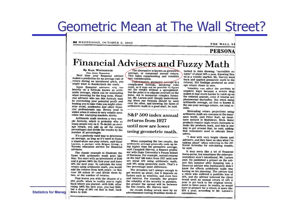
Geometric Mean at The Wall Street? D2 WEDNESDAY.OCTOBER 8.2003 THE WALL ST PERSONA Financial Advisers and Fuzzy Math ng ced an aver arithmetie math is a good start,he said. ar ave a S&P 500 index annual returns from 1927 三品8妙然 sts to de an aver until now are lower using geometric math. It's a pe to the Fot te the total h,Thts3 ret mns from in thus them by but it depenc ion of a ate back wh rvey 6 Statistics for Ma
Statistics for Managers Using Microsoft Excel Chap 3-19 Geometric Mean at The Wall Street?

Geometrical Mean:Example An investment of $100,000 declined to $50,000 at the end of year one and rebounded to $100,000 at end of year two: X1=$100,000X2=$50,000X3=$100,000 50%decrease 100%increase The overall two-year return is zero,since it started and ended at the same level. Statistics for Mar nagers Using Microsoft Excel Chap 3-20
Statistics for Managers Using Microsoft Excel Chap 3-20 Geometrical Mean: Example An investment of $100,000 declined to $50,000 at the end of year one and rebounded to $100,000 at end of year two: The overall two-year return is zero, since it started and ended at the same level. X1 $100,000 X2 $50,000 X3 $100,000 50% decrease 100% increase