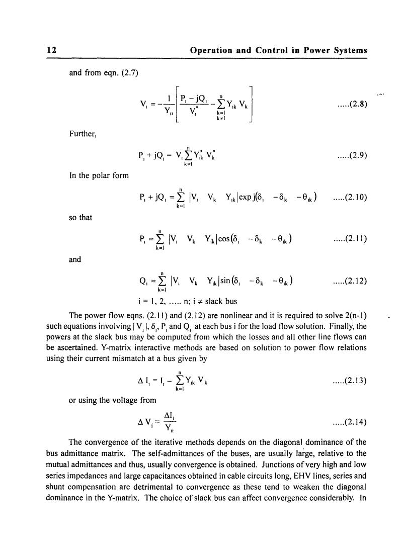
12 Operation and Control in Power Systems and from eqn.(2.7) (2.8) Further, P+jQ-V>YiV: ..(2.9) In the polar form R+0,=玄V.Yalep6-8:-0 )(2.10) so that P.V.V:Yalcos(6,-0) .(2.11) and Q.V.V.Yalsin(6,8x0x ..(2.12) k=1 i=1,2,.n;i≠slack bus The power flow eqns.(2.11)and(2.12)are nonlinear and it is required to solve 2(n-1) such equations involving V,,P and Q at each bus i for the load flow solution.Finally,the powers at the slack bus may be computed from which the losses and all other line flows can be ascertained.Y-matrix interactive methods are based on solution to power flow relations using their current mismatch at a bus given by A,=-} .(2.13) or using the voltage from △V=Y .(2.14) The convergence of the iterative methods depends on the diagonal dominance of the bus admittance matrix.The self-admittances of the buses,are usually large,relative to the mutual admittances and thus,usually convergence is obtained.Junctions of very high and low series impedances and large capacitances obtained in cable circuits long,EHV lines,series and shunt compensation are detrimental to convergence as these tend to weaken the diagonal dominance in the Y-matrix.The choice of slack bus can affect convergence considerably.In
12 Operation and Control in Power Systems and from eqn. (2.7) ..... (2.8) Further, n P, + jQ, = V, LYi~ V: ..... (2.9) k=1 In the polar form n P, + jQ, = L lV, Vk Y,klexpj(o, -Ok -e,k) ..... (2.10) k=1 so that n P, == L lV, Vk Yiklcos(o, -Ok -e,k) ..... (2.11 ) k=1 and n Q, == L lV, Vk Y,k Isin (0, -Ok -e,k) ..... (2.12) k=1 i = 1, 2, ..... n; i -:t:- slack bus The power flow eqns. (2.11) and (2.12) are nonlinear and it is required to solve 2(n-1) such equations involving 1 V, I, 0" P, and Q, at each bus i for the load flow solution. Finally, the powers at the slack bus may be computed from which the losses and all other line flows can be ascertained. V-matrix interactive methods are based on solution to power flow relations using their current mismatch at a bus given by n L\ I, = I, - L Y,k V k k=1 or using the voltage from L\I· L\ V.==-' I YII ..... (2.13) ..... (2.14) The convergence of the iterative methods depends on the diagonal dominance of the bus admittance matrix. The self-admittances of the buses, are usually large, relative to the mutual admittances and thus, usually convergence is obtained. Junctions of very high and low series impedances and large capacitances obtained in cable circuits long, EHV lines, series and shunt compensation are detrimental to convergence as these tend to weaken the diagonal dominance in the V-matrix. The choice of slack bus can affect convergence considerably. In

Load Flow Analysis 13 difficult cases,it is possible to obtain convergence by removing the least diagonally dominant row and column of Y.The salient features of the Y-matrix iterative methods are that the elements in the summation terms in egn.(2.7)or(2.8)are on the average only three even for well-developed power systems.The sparsity of the Y-matrix and its symmetry reduces both the storage requirement and the computation time for iteration (sec.4).For a large,well conditioned system of n-buses,the number of iterations required are of the order of n and total computing time varies approximately as n2. Instead of using eqn(2.6),one can select the impedance matrix and rewrite the equation as V=Y-II=Z.I ..(2.15) The Z-matrix method is not usually very sensitive to the choice of the slack bus.It can easily be verified that the Z-matrix is not sparse.For problems that can be solved by both Z-matrix and Y-matrix methods,the former are rarely competitive with the Y-matrix methods. 2.3 Gauses-Seidel Iterative Method In this method,voltages at all buses except at the slack bus are assumed.The voltage at the slack bus is specified and remains fixed at that value.The (n-1)bus voltage relations. P.-iQ ..(2.16) i=l,2,.n;i≠slack bus are solved simultaneously for an improved solution.In order to accelerate the convergence,all newly-computed values of bus voltages are substituted in eqn.(2.16).The bus voltage equation of the(m+1)th iteration may then be written as P,-jQ, .(2.17) Vm产 k=1 k The method converges slowly because of the loose mathematical coupling between the buses.The rate of convergence of the process can be increased by using acceleration factors to the solution obtained after each iteration.A fixed acceleration factor a (I s a s 2)is normally used for each voltage change, AV =a- S .(2.18)
Load Flow Analysis 13 difficult cases, it is possible to obtain convergence by removing the least diagonally dominant row and column of Y. The salient features of the V-matrix iterative methods are that the elements in the summation terms in eqn. (2.7) or (2.8) are on the average only three even for well-developed power systems. The sparsity of the V-matrix and its symmetry reduces both the storage requirement and the computation time for iteration (sec. 4). For a large, well conditioned system of n-buses, the number of iterations required are of the order of n and total computing time varies approximately as n2• Instead of using eqn (2.6), one can select the impedance matrix and rewrite the equation as v = y-I 1= Z.I ..... (2.15) The Z-matrix method is not usually very sensitive to the choice of the slack bus. It can easily be verified that the Z-matrix is not sparse. For problems that can be solved by both Z-matrix and V-matrix methods, the former are rarely competitive with the V-matrix methods. 2.3 Gauses - Seidel Iterative Method In this method, voltages at all buses except at the slack bus are assumed. The voltage at the slack bus is specified and remains fixed at that value. The (n-I) bus voltage relations. V=_I [pl-jQI-~Y v] I Y V· L. Ik k II I k=1 k",] ..... (2.16) i = I, 2, ..... n; i 7= slack bus are solved simultaneously for an improved solution. In order to accelerate'the convergence, all newly-computed values of bus voltages are substituted in eqn. (2.16). The bus voltage equation of the (m + I )th iteration may then be written as ..... (2.17) The method converges ~low1y because of the loose mathematical coupling between the buses. The rate of convergence of the process can be increased by using acceleration factors to the solution obtained after each iteration. A fixed acceleration factor a (I ::; a ::; 2) is normally used for each voltage change, AV = a AS: I • VjYII ..... (2.18)
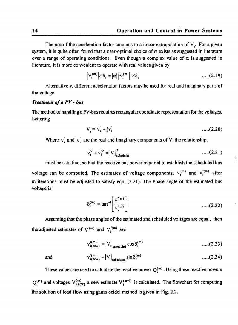
14 Operation and Control in Power Systems The use of the acceleration factor amounts to a linear extrapolation of V.For a given system,it is quite often found that a near-optimal choice of a exists as suggested in literature over a range of operating conditions.Even though a complex value of a is suggested in literature,it is more convenient to operate with real values given by vm,=laYm|∠, (2.19) Alternatively,different acceleration factors may be used for real and imaginary parts of the voltage. Treatment of a PV-bus The method of handling a PV-bus requires rectangular coordinate representation for the voltages. Lettering V=v,+jv, .(2.20) Where v;and v,are the real and imaginary components of V the relationship. V abedulea (2.21) must be satisfied,so that the reactive bus power required to establish the scheduled bus voltage can be computed.The estimates of voltage components,v(m)and vm)after m iterations must be adjusted to satisfy eqn.(2.21).The Phase angle of the estimated bus voltage is δm)=tan v .(2.22) Assuming that the phase angles of the estimated and scheduled voltages are equal,then the adjusted estimates of vm)and Vm)are v,=Vδam .(2.23) and Vchoduded sinm) (2.24) These values are used to calculate the reactive power Qm).Using these reactive powers Qand voltages Vanew estimate V)is calculated.The flowchart for computing the solution of load flow using gauss-seidel method is given in Fig.2.2
14 Operation and Control in Power Systems The use of the acceleration factor amounts to a linear extrapolation of VI' For a given system, it is quite often found that a near-optimal choice of a exists as suggested in literature over -a range of operating conditions. Even though a complex value of a is suggested in literature, it is more convenient to operate with real values given by ..... (2.19) Alternatively, different acceleration factors may be used for real and imaginary parts of the voltage. Treatment of a PV - bus The method of handling a PV -bus requires rectangular coordinate representation for the voltages. Lettering ..... (2.20) Where v; and v;' are the real and imaginary components of Vi the relationship. V '2 +v· "2 ::; 1 V 12 I I I schedules ..... (2.21) must be satisfied, so that the reactive bus power required to establish the scheduled bus voltage can be computed. The estimates of voltage components, v;(m) and V;-(m) after m iterations must be adjusted to satisfy eqn. (2.21). The Phase angle of the estimated bus voltage is [ "Cm) 1 oem) I = tan-I ~ 'em) Vi ..... (2.22) Assuming that the phase angles of the estimated and scheduled voltages are equal; .then the adjusted estimates of V'(m) and V;'cm) are ICm) -IV I s:Cm) vi(new) - I Scheduiedcosul ..... (2.23) and "(m) _I I . (m) vi(new) - VlscheduledsmBj ..... (2.24) These values are used to calculate the reactive power Q\m) . Using these reactive powers Q~m) and voltages Vi\~~W) a new estimate V lm+l) is calculated. The flowchart for computing the solution of load flow using gauss-seidel method is given in Fig. 2.2
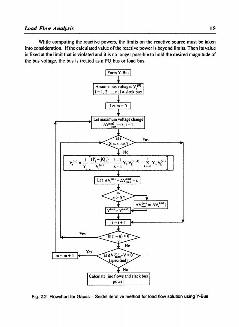
Load Flow Analysis 15 While computing the reactive powers,the limits on the reactive source must be taken into consideration.If the calculated value of the reactive power is beyond limits.Then its value is fixed at the limit that is violated and it is no longer possible to hold the desired magnitude of the bus voltage,the bus is treated as a PQ bus or load bus. Form Y-Bus Assume bus voltages V(0) i=1.2n:i≠slack bus Let m=0 Let maximum voltage change AV(mx-0:i=1 isi Yes Slack bus No vim)=_ 1 (P-j0)i-1 y(m) k= Ya VimD-YaVi) k=i+l Let AV(m)-AVm= ∈>02 v(m)=V(m-1) i=i+1 Yes is(i-n)≤0 No Yes m=m+1 isAV(m-V>0 (specified) 立No Calculate line flows and slack bus power Fig.2.2 Flowchart for Gauss-Seidel iterative method for load flow solution using Y-Bus
Load Flow Analysis 15 While computing the reactive powers, the limits on the reactive source must be taken into consideration. If the calculated value of the reactive power is beyond limits. Then its value is fixed at the limit that is violated and it is no longer possible to hold the desired magnitude of the bus voltage, the bus is treated as a PQ bus or load bus. Yes VCm ) =_1 [<PJ-.iQJ) ~Y v(m+l)_ i Y VIm)] 1 Y Vcm) k = 1 Ik k k=I+1 Ik k IJ 1 Yes m=m+ 1 Yes Calculate line flows and slack bus power Fig. 2.2 Flowchart for Gauss - Seidel iterative method for load flow solution using Y-Bus
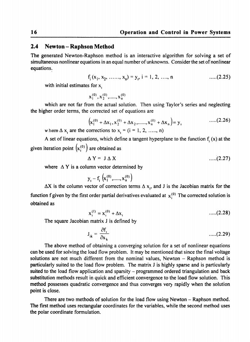
16 Operation and Control in Power Systems 2.4 Newton-Raphson Method The generated Newton-Raphson method is an interactive algorithm for solving a set of simultaneous nonlinear equations in an equal number of unknowns.Consider the set of nonlinear equations. f(x1,X2,,x)=ypi=1,2,,n ..…(2.25) with initial estimates for x, x0,x9,,x0 which are not far from the actual solution.Then using Taylor's series and neglecting the higher order terms,the corrected set of equations are )+x)x+Ax)=y (2.26) w here△x,are the corrections to x,=(i=l,2,,n) A set of linear equations,which define a tangent hyperplane to the function f(x)at the given iteration point xare obtained as △Y=J△X .(2.27) where A Y is a column vector determined by y,-£k0,x0) AX is the column vector of correction terms A x,,and J is the Jacobian matrix for the function fgiven by the first order partial derivatives evaluated at xThe corrected solution is obtained as x"=x0+△x .(2.28) The square Jacobian matrix J is defined by of, Jik0x ..(2.29) The above method of obtaining a converging solution for a set of nonlinear equations can be used for solving the load flow problem.It may be mentioned that since the final voltage solutions are not much different from the nominal values,Newton-Raphson method is particularly suited to the load flow problem.The matrix J is highly sparse and is particularly suited to the load flow application and sparsity-programmed ordered triangulation and back substitution methods result in quick and efficient convergence to the load flow solution.This method possesses quadratic convergence and thus converges very rapidly when the solution point is close. There are two methods of solution for the load flow using Newton-Raphson method. The first method uses rectangular coordinates for the variables,while the second method uses the polar coordinate formulation
16 Operation and Control in Power Systems 2.4 Newton - Raphson Method The generated Newton-Raphson method is an interactive algorithm for solving a set of simultaneous nonlinear equations in an equal number of unknowns. Consider the set of nonlinear equations: fj (xl' x2' ...... , xn) = YI' i = 1,2, .... , n ..... (2.25) with initial estimates for XI (0) (0) (0) XI ,x2 , ••••• , xn which are not far from the actual solution. Then using Taylor's series and neglecting the higher order terms, the corrected set of equations are (X\O) + ~XI' x~O) + ~X2 , ...... , <0) + ~xn)= YI ..... (2.26) w here ~ XI are the corrections to X. = (i = I, 2, ..... , n) A set of linear equations, which define a tangent hyperplane to the function ~ (x) at the given iteration point (x~O») are obtained as ~Y= J~X ..... (2.27) where ~ Y is a column vector determined by YI _ ~ (x\O) , ..... ,x~O») ~X is the column vector of correction terms ~ XI' and J is the Jacobian matrix for the function f given by the first order partial derivatives evaluated at x~O) The corrected solution is obtained as X(I) = x(O) + ~X I I I ..... (2.28) The square Jacobian matrix J is defined by Ofl Jlk = Ox k ..... (2.29) The above method of obtaining a converging solution for a set of nonlinear equations can be used for solving the load flow problem. It may be mentioned that since the final voltage solutions are not much different from the nominal values, Newton - Raphson method is particularly suited to the load flow problem. The matrix J is highly sparse and is particularly suited to the load flow application and sparsity - programmed ordered triangulation and back substitution methods result in quick and efficient convergence to the load flow solution. This method possesses quadratic convergence and thus converges very rapidly when the solution point is close. There are two methods of solution for the load flow using Newton - Raphson method. The first method uses rectangular coordinates for the variables, while the second method uses the polar coordinate formulation