Introduction 7 by allowing the phase angle between the two end voltages 8,to change.This is brought about by adjusting the throttle of the prime movers in the generating stations at one end or both ends of the line.The pewer transfer over the line is given by P-VsVe.sin X where Vs and Ve are sending end and receiving end voltage magnitudes respectively. By slowly increasing the load,the maximum power transfer can be obtained when 900.Further,increase in load will not increase the power transmitted,but instead decreases it.This point is referred to as the static stability limit or static transmission capacity of the line. This capacity can,of course,be increased by increasing the voltage magnitudes,but there are limits for this increase. The incremental increase in transmitted power AP caused by a small increment A8 in the phase angle is a measure of the electrical stiffness of the transmission line.The quantity △P is also called synchronizing coefficient. It can be seen that the transmission capacity can be increased also by reducing the effective reactance of the line.This can be achieved by paralleling the lines,using bundled conductors or inserting series capacitors. The analysis,operation and control of inter connected power systems or simply areas are discussed comprehensively in Chapter 7.The objective of system voltage control is to maintain a satisfactory voltage profile in the system during both periods of maximum and minimum loadings.A detailed analysis of excitation control and means adopted for reactive power generation in addition to synchronous machine are presented in Chapter 8. Various devices such as tap changers,reactors,capacitors,induction regulators static var compensators etc.,are discussed in Chapter 8.The role of a power system stabilizer is also presented. In Chapter 9,certain advanced topics that are related to operation and control are introduced.These are,state estimation,FACTS controllers,Voltage stability,Power quality, load prediction,energy control centers etc.The inclusion of the topics and the presentation of the information is by no means exhaustive
IntrtJduction 7 by allowing the phase angle between the two end voltages 0, to change. This is brought about by adjusting the throttle ofthe prime movers in the generating stations at one end or both ends of the line. The pewer transfer over the line is given by p=VsVRSino XL where V s and V R are sending end and receiving end voltage magnitudes respectively. By slowly increasing the load, the maximum power transfer can be obtained when o ~ 90°. Further, increase in load will not increase the power transmitted, but instead decreases it. This point is referred to as the static stability limit or static transmission capacity of the line. This capacity can, of course, be increased by increasing the voltage magnitudes, but there are limits for this increase. The incremental increase in transmitted power ~p caused by a small increment ~o in the phase angle is a measure of the electrical stiffness of the transmission line. The quantity (~) is also called synchronizing coefficient. It can be seen that the transmission capacity can be increased also by reducing the effective reactance of the line. This can be achieved by paralleling the lines, using bundled conductors or inserting series capacitors. The analysis, operation and control of inter connected power systems or simply areas are discussed comprehensively in Chapter 7. The objective of system voltage control is to maintain a satisfactory voltage profile in the system during both periods of maximum and minimum loadings. A detailed analysis of excitation control and means adopted for reactive power generation in addition to synchronous machine are presented in Chapter 8. Various devices such as tap changers, reactors, capacitors, induction regulators static var compensators etc., are discussed in Chapter 8. The role of a power system stabilizer is also presented. In Chapter 9, certain advanced topics that are related to operation and control are introduced. These are, state estimation, FACTS controllers, Voltage stability, Power quality, load prediction, energy control centers etc. The inclusion of the topics and the presentation of the information is by no means exhaustive
2 LOAD FLOW ANALYSIS Load Flow or Power Flow is the solution for the Power System under static conditions of operation.Load Flow studies are undertaken to determine 1.The line flows 2.The bus voltages and system voltage profile 3.The effect of changes in circuit configuration,and incorporating new circuits on system loading 4.The effect of temporary loss of transmission capacity and(or)generation on system loading and accompanied effects 5.The effect of in-phase and quadrature boost voltages on system loading. 6.Economic system operation 7.system transmission loss minimization 8.Transformer tap settings for economic operation and 9.Possible improvements to an existing system by change of conductor sizes and system voltages. For the purpose of load flow studies,a single phase representation of the power network is used since the system is generally balanced.When systems had not grown to the present size,networks were simulated on network analyzers for power flow studies.These analyzers
2 LOAD FLOW ANALYSIS Load Flow or Power Flow is the solution for the Power System under static conditions of operation. Load Flow studies are undertaken to determine: I. The line flows 2. The bus voltages and system voltage profile 3. The effect of changes in circuit configuration, and incorporating new circuits on system loading 4. The effect of temporary loss of transmission capacity and (or) generation on system loading and accompanied effects 5. The effect of in-phase and quadrature boost voltages on system loading. 6. Economic system operation 7. system transmission loss minimization 8. Transformer tap settings for economic operation and 9. Possible improvements to an existing system by change of conductor sizes and system voltages. For the purpose of load flow studies, a single phase representation of the power network is used since the system is generally balanced. When systems had not grown to the present size, networks were simulated on network analyzers for power flow studies. These analyzers
Load Flow Analysis 9 are of analogue type,scaled down miniature models of power systems with resistances, reactances,capacitances,autotransformers,transformers,loads,and generators.The generators are just supply sources operating at a much higher frequency than 50Hz to limit the size of the components.The loads are represented by constant impedances.Meters are provided on the panel board for measuring voltages,currents,and powers.The load flow solution is obtained directly from measurements for any system simulated on the analyzer. With the advent of the modern digital computer possessing large storage and high speed, the mode of load flow studies have changed from analog to digital simulation.A large number of algorithms are developed for digital power flow solutions.Some of the generally used methods are described in this chapter.The methods basically distinguish between themselves in the rate of convergence,storage requirement and time of computation.The loads are generally represented by constant power. In the network at each bus or node there are four variables viz. (① Voltage magnitude (i) Voltage phase angle (iii)Real power and (iv)Reactive power. Out of these four quantities two of them are specified at each bus and the remaining two are determined from the load flow solution.To supply the real and reactive power losses in lines which will not be known till the end of the power flow solution,a generator bus,called slack or swing bus is selected.At this bus,the generator voltage magnitude and its phase angle are specified so that the unknown power losses are also assigned to this bus in addition to balance of generation if any.Generally,at all other buses,voltage magnitude and real power are specified.At all load buses the real and the reactive load demands are specified.Table 2.1 illustrates the types of buses and the associated known and unknown variables. 2.1 Bus Classification Table 2.1 Bus Specified variables Computed variables Slack-bus Voltage magnitude and its phase angle Real and reactive powers Generator bus Magnitudes of bus voltages and real Voltage phase angle and (PV-bus or voltage powers(limit on reactive powers) reactive power. controlled bus) Load bus Real and reactive powers Magnitude and phase angle of bus voltages
Load Flow Analysis 9 are of analogue type, scaled down miniature models of power systems with resistances, reactances, capacitances, autotransformers, transformers, loads, and generators. The generators are just supply sources operating at a much higher frequency than 50Hz to limit the size of the components. The loads are represented by constant impedances. Meters are provided on the panel board for measuring voltages, currents, and powers. The load flow solution is obtained directly from measurements for any system simulated on the analyzer. With the advent of the modern digital computer possessing large storage and high speed, the mode of load flow studies have changed from analog to digital simulation. A large number of algorithms are developed for digital power flow solutions. Some of the generally used methods are described in this chapter. The methods basically distinguish between themselves in the rate of convergence, storage requirement and time of computation. The loads are generally represented by constant power. In the network at each bus or node there are four variables viz. (i) Voltage magnitude (ii) Voltage phase angle (iii) Real power and (iv) Reactive power. Out of these four quantities two of them are specified at each bus and the remaining two are determined from the load flow solution. To supply the real and reactive power losses in lines which will not be known till the end of the power flow solution, a generator bus, called slack or swing bus is selected. At this bus, the gen~rator voltage magnitude and its phase angle are specified so that the unknown power losses are also assigned to this bus in addition to balance of generation if any. Generally, at all other buses, voltage magnitude and real power are specified. At all load buses the real and the reactive load demands are specified. Table 2.1 illustrates the types of buses and the associated known and unknown variables. 2.1 Bus Classification Table 2.1 Bus Specified variables Computed variables Slack - bus Voltage magnitude and its phase angle Real and reactive powers Generator bus Magnitudes of bus voltages and real Voltage phase angle and (PV - bus or voltage powers (limit on reactive powers) reactive power. controlled bus) Load bus Real and reactive powers Magnitude and phase angle of bus voltages
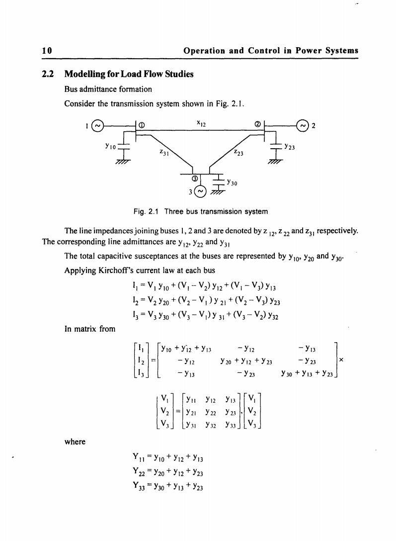
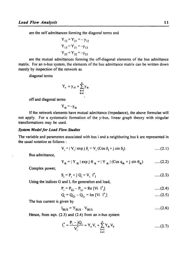
10 Operation and Control in Power Systems 2.2 Modelling for Load Flow Studies Bus admittance formation Consider the transmission system shown in Fig.2.1. ① X12 Z31 223 ③ 3⊙易 Fig.2.1 Three bus transmission system The line impedances joining buses 1,2 and 3 are denoted by z2 andz respectively. The corresponding line admittances are y2 y22 and y3 The total capacitive susceptances at the buses are represented by yoy2o and y3o. Applying Kirchoff's current law at each bus I1=V1y1o+(V,-V2)y12+(V1-V)y13 l2=V2y20+(V2-V1)y21+(V2-V,)y23 I3=V3y30+(V3-V)y31+(V3-V2)y32 In matrix from y1o +yi2 +y13 -y12 -y13 -y2 y20+y12+y23 -y23 -y13 -y23 y30+y13+y23」 yu y12 yi3 y22 y23 V3 y31 y32 where Y11=y10+y12+y13 Y2=y20+y12+y23 Y33=y30+y13+y23
10 Operation and Control in Power Systems 2.2 Modelling for Load Flow Studies Bus admittance formation Consider the transmission system shown in Fig. 2.1. Fig. 2.1 Three bus transmission system The line impedances joining buses 1,2 and 3 are denoted by z 12' Z 22 and z31 respectively. The corresponding line admittances are Y12' Y22 and Y31 The total capacitive susceptances at the buses are represented by YIO' Y20 and Y30' Applying Kirchoff's current law at each bus In matrix from where II = VI YIO + (VI - V2) YI2 + (VI - V3) YI3 12 = V2 Y20 + (V2 - VI) Y 21 + (V2 - V3) Y23 13 = V3 Y30 + (V3 - VI) Y 31 + (V3 - V2) Y32 lll] 12 f' _. +!I' Y 12 + y" 13 -YI3 l VI] [YII V2 == Y2I V3 YJI YII == YIO + YI2 + YI3 Y22 = Y20 + YI2 + Y23 Y33 = Y30 + YI3 + Y23 YI2 Y22 Y32 - YI2 Y 20 + Y 12 + Y 23 - Y23 Y23 y"]n ' ~2 Y 33 3 - Y13 ] - Y23 x Y30 + YI3 + Y23
Load Flow Analysis 11 are the self admittances forming the diagonal terms and Y12=Y21=-y12 Y13=Y31=-y13 Y23=Y32=-y23 are the mutual admittances forming the off-diagonal elements of the bus admittance matrix.For an n-bus system,the elements of the bus admittance matrix can be written down merely by inspection of the network as diagonal terms Ym=yio+ k= off and diagonal terms Yik=-yik If the network elements have mutual admittance(impedance),the above formulae will not apply.For a systematic formation of the y-bus,linear graph theory with singular transformations may be used. System Model for Load Flow Studies The variable and parameters associated with bus i and a neighboring bus k are represented in the usual notation as follews V,=|V,l expjδ,=V,(Cosδ,+jsinδ) .(2.1) Bus admittance, Yik=IY ik l exp j0 k=Y k (Cos qik +j sin 0k) .(2.2) Complex power, S=P+j=Vi I' ..(2.3) Using the indices G and L for generation and load, P,=PGI PLi=Re [Vi I'] (2.4) Q=QG -QL Im [Vi I'] ..(2.5) The bus current is given by IBus YBUs.VBus .(2.6) Hence,from eqn.(2.3)and(2.4)from an n-bus system i-B-iQ.-Y.V.+ZY.V …(2.7) k=1
Load Flow Analysis are the self admittances forming the diagonal terms and Y12 =Y21 =-YI2 Y 13 =Y31 =-YI3 Y 23 = Y 32 = -Y23 11 are the mutual admittances forming the off-diagonal elements of the bus admittance matrix. For an n-bus system, the elements of the bus admittance matrix can be written down merely by inspection of the network as diagonal terms n YII = YiO + LY,k k=1 k .. i off and diagonal terms Y.k =-Y.k If the network elements have mutual admittance (impedance), the above formulae wi\l not apply. For a systematic formation of the y-bus, linear graph theory with singular transformations may be used. System Model for Load Flow Studies The variable and parameters associated with bus i and a neighboring bus k are represented in the usual notation as follows : Bus admittance, Y.k = I Y ik I exp j e .k = I Y .k I (Cos q.k + j sin e.k) Complex power, S. = p. + j Q. = Vi [\ Using the indices G and L for generation and load, p. = PG• - PLi = Re [Vi [.J Q. = QG. - QL. = 1m [Vi 1.1 ] The bus current is given by IBus = Y BUS . V BUS Hence, from eqn. (2.3) and (2.4) from an n-bus system I ~ = P, - jQ I Y ~ I V,. = II V, + L Y,k V k I k=1 k .. 1 ..... (2.1 ) ..... (2.2) ..... (2.3) ..... (2.4) ..... (2.5) ..... (2.6) ..... (2.7)