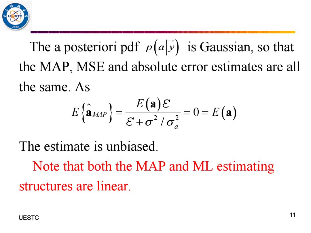
The a posteriori pdf p(a)i is Gaussian,so that the MAP.MSE and absolute error estimates are all the same.As sawE4go5。 E) =0=E(a) The estimate is unbiased. Note that both the MaP and ML estimating structures are linear. UESTC 11
The a posteriori pdf is Gaussian, so that the MAP, MSE and absolute error estimates are all the same. As The estimate is unbiased. Note that both the MAP and ML estimating structures are linear. 11 UESTC p a y ( ) ( ) ( ) 2 2 0 / MAP a E E E a a a = = = + ε ε

MAC 8+ aMAP Sample ↑every Si k cycles Figure 11.2.MAP structure for coherent estimation of amplitude MAC 是 A L Sample every Si k cycles Figure 11.3.ML structure for coherent estimation of amplitude UESTC 12
12 UESTC

The continuous form of the ML estimate is a=y0(oh 1 where E-[s()d And a continuous form of the MAP estimate form 1S 入 ()(d E+ UESTC 13
The continuous form of the ML estimate is where And a continuous form of the MAP estimate form is 13 UESTC ( ) ( ) 0 1 T ML = t s t dt a y ε ( ) 2 0 T s t dt ε= ( ) ( ) 0 0 2 1 2 T MAP t s t dt N = + a a y ε

11.5 Amplitude estimation in the noncoherent case with WGN Assume the signal is sinusoidal with an unknown carrier phase uniformly distributed in (0,2).The measured signal is then represented by y,=asin(2πfiT,+8)+n,1≤i≤k As n,is zero-mean,white Gaussian noise random variable with varianceo2,we have B=2πfT, a0gon2L-ana) UESTC
11.5 Amplitude estimation in the noncoherent case with WGN Assume the signal is sinusoidal with an unknown carrier phase uniformly distributed in . The measured signal is then represented by As is zero-mean, white Gaussian noise random variable with variance , we have 14 UESTC (0,2 ) y a n i s i = + + sin 2 , 1 ( f iT i k 0 ) ni 2 ( ) ( ) ( ) 2 / 2 2 2 1 1 1 , exp sin 2 2 k k i i p y a y a i = = − − + 0 2 s = f T