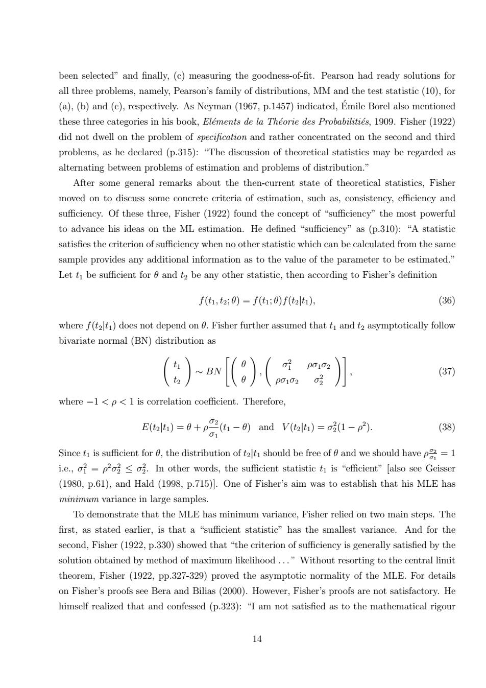
been selected"and finally,(c)measuring the goodness-of-fit.Pearson had ready solutions for all three problems,namely,Pearson's family of distributions,MM and the test statistic(10),for (a),(b)and (c),respectively.As Neyman (1967,p.1457)indicated,Emile Borel also mentioned these three categories in his book,Elements de la Theorie des Probabilities,1909.Fisher(1922) did not dwell on the problem of specification and rather concentrated on the second and third problems,as he declared(p.315):"The discussion of theoretical statistics may be regarded as alternating between problems of estimation and problems of distribution." After some general remarks about the then-current state of theoretical statistics,Fisher moved on to discuss some concrete criteria of estimation,such as,consistency,efficiency and sufficiency.Of these three,Fisher (1922)found the concept of "sufficiency"the most powerful to advance his ideas on the ML estimation.He defined "sufficiency"as (p.310):"A statistic satisfies the criterion of sufficiency when no other statistic which can be calculated from the same sample provides any additional information as to the value of the parameter to be estimated." Let t be sufficient for 0 and t2 be any other statistic,then according to Fisher's definition f(t,t2;9)=f(t1;0)f(t2lt), (36) where f(t2t1)does not depend on 0.Fisher further assumed that ti and t2 asymptotically follow bivariate normal(BN)distribution as (37) where-1<p<1 is correlation coefficient.Therefore, E(tat)=0+p22(t-0)and V(talh)=o(1-p). (38) 01 Sincet is sufficient for0,the distribution of t should be free of and we should have p=1 i.e.,o?=p22o2.In other words,the sufficient statistic t is"efficient"[also see Geisser (1980,p.61),and Hald (1998,p.715).One of Fisher's aim was to establish that his MLE has minimum variance in large samples. To demonstrate that the MLE has minimum variance,Fisher relied on two main steps.The first,as stated earlier,is that a "sufficient statistic"has the smallest variance.And for the second,Fisher(1922,p.330)showed that "the criterion of sufficiency is generally satisfied by the solution obtained by method of maximum likelihood..."Without resorting to the central limit theorem,Fisher (1922,pp.327-329)proved the asymptotic normality of the MLE.For details on Fisher's proofs see Bera and Bilias(2000).However,Fisher's proofs are not satisfactory.He himself realized that and confessed (p.323):"I am not satisfied as to the mathematical rigour 14
been selected” and finally, (c) measuring the goodness-of-fit. Pearson had ready solutions for all three problems, namely, Pearson’s family of distributions, MM and the test statistic (10), for (a), (b) and (c), respectively. As Neyman (1967, p.1457) indicated, Emile Borel also mentioned ´ these three categories in his book, El´ements de la Th´eorie des Probabiliti´es, 1909. Fisher (1922) did not dwell on the problem of specification and rather concentrated on the second and third problems, as he declared (p.315): “The discussion of theoretical statistics may be regarded as alternating between problems of estimation and problems of distribution.” After some general remarks about the then-current state of theoretical statistics, Fisher moved on to discuss some concrete criteria of estimation, such as, consistency, efficiency and sufficiency. Of these three, Fisher (1922) found the concept of “sufficiency” the most powerful to advance his ideas on the ML estimation. He defined “sufficiency” as (p.310): “A statistic satisfies the criterion of sufficiency when no other statistic which can be calculated from the same sample provides any additional information as to the value of the parameter to be estimated.” Let t1 be sufficient for θ and t2 be any other statistic, then according to Fisher’s definition f(t1, t2; θ) = f(t1; θ)f(t2|t1), (36) where f(t2|t1) does not depend on θ. Fisher further assumed that t1 and t2 asymptotically follow bivariate normal (BN) distribution as t1 t2 ! ∼ BN " θ θ ! , σ 2 1 ρσ1σ2 ρσ1σ2 σ 2 2 !# , (37) where −1 < ρ < 1 is correlation coefficient. Therefore, E(t2|t1) = θ + ρ σ2 σ1 (t1 − θ) and V (t2|t1) = σ 2 2 (1 − ρ 2 ). (38) Since t1 is sufficient for θ, the distribution of t2|t1 should be free of θ and we should have ρ σ2 σ1 = 1 i.e., σ 2 1 = ρ 2σ 2 2 ≤ σ 2 2 . In other words, the sufficient statistic t1 is “efficient” [also see Geisser (1980, p.61), and Hald (1998, p.715)]. One of Fisher’s aim was to establish that his MLE has minimum variance in large samples. To demonstrate that the MLE has minimum variance, Fisher relied on two main steps. The first, as stated earlier, is that a “sufficient statistic” has the smallest variance. And for the second, Fisher (1922, p.330) showed that “the criterion of sufficiency is generally satisfied by the solution obtained by method of maximum likelihood . . . ” Without resorting to the central limit theorem, Fisher (1922, pp.327-329) proved the asymptotic normality of the MLE. For details on Fisher’s proofs see Bera and Bilias (2000). However, Fisher’s proofs are not satisfactory. He himself realized that and confessed (p.323): “I am not satisfied as to the mathematical rigour 14

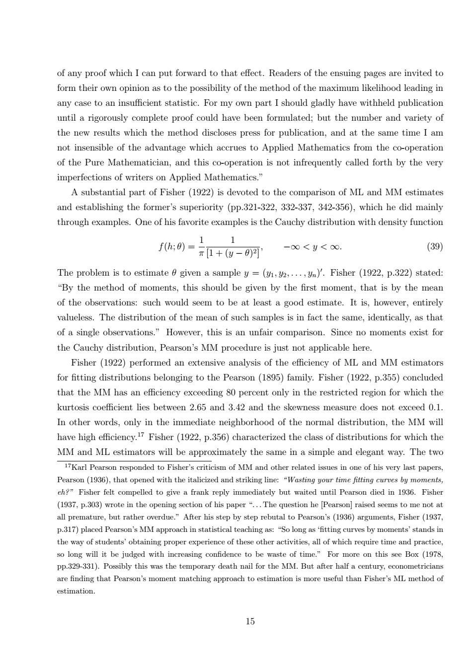
of any proof which I can put forward to that effect.Readers of the ensuing pages are invited to form their own opinion as to the possibility of the method of the maximum likelihood leading in any case to an insufficient statistic.For my own part I should gladly have withheld publication until a rigorously complete proof could have been formulated;but the number and variety of the new results which the method discloses press for publication,and at the same time I am not insensible of the advantage which accrues to Applied Mathematics from the co-operation of the Pure Mathematician,and this co-operation is not infrequently called forth by the very imperfections of writers on Applied Mathematics." A substantial part of Fisher (1922)is devoted to the comparison of ML and MM estimates and establishing the former's superiority (pp.321-322,332-337,342-356),which he did mainly through examples.One of his favorite examples is the Cauchy distribution with density function fh:0)=11 -∞<y<∞. (39) π[1+(g-)2] The problem is to estimate 0 given a sample y=(v1,22,...,Un).Fisher (1922,p.322)stated: "By the method of moments,this should be given by the first moment,that is by the mean of the observations:such would seem to be at least a good estimate.It is,however,entirely valueless.The distribution of the mean of such samples is in fact the same,identically,as that of a single observations."However,this is an unfair comparison.Since no moments exist for the Cauchy distribution,Pearson's MM procedure is just not applicable here. Fisher (1922)performed an extensive analysis of the efficiency of ML and MM estimators for fitting distributions belonging to the Pearson (1895)family.Fisher (1922,p.355)concluded that the MM has an efficiency exceeding 80 percent only in the restricted region for which the kurtosis coefficient lies between 2.65 and 3.42 and the skewness measure does not exceed 0.1. In other words,only in the immediate neighborhood of the normal distribution,the MM will have high efficiency.17 Fisher(1922,p.356)characterized the class of distributions for which the MM and ML estimators will be approximately the same in a simple and elegant way.The two 17Karl Pearson responded to Fisher's criticism of MM and other related issues in one of his very last papers, Pearson(1936),that opened with the italicized and striking line:"Wasting your time fitting curves by moments, eh?"Fisher felt compelled to give a frank reply immediately but waited until Pearson died in 1936.Fisher (1937,p.303)wrote in the opening section of his paper "..The question he [Pearson]raised seems to me not at all premature,but rather overdue."After his step by step rebutal to Pearson's(1936)arguments,Fisher(1937, p.317)placed Pearson's MM approach in statistical teaching as:"So long as fitting curves by moments'stands in the way of students'obtaining proper experience of these other activities,all of which require time and practice, so long will it be judged with increasing confidence to be waste of time."For more on this see Box(1978, pp.329-331).Possibly this was the temporary death nail for the MM.But after half a century,econometricians are finding that Pearson's moment matching approach to estimation is more useful than Fisher's ML method of estimation. 15
of any proof which I can put forward to that effect. Readers of the ensuing pages are invited to form their own opinion as to the possibility of the method of the maximum likelihood leading in any case to an insufficient statistic. For my own part I should gladly have withheld publication until a rigorously complete proof could have been formulated; but the number and variety of the new results which the method discloses press for publication, and at the same time I am not insensible of the advantage which accrues to Applied Mathematics from the co-operation of the Pure Mathematician, and this co-operation is not infrequently called forth by the very imperfections of writers on Applied Mathematics.” A substantial part of Fisher (1922) is devoted to the comparison of ML and MM estimates and establishing the former’s superiority (pp.321-322, 332-337, 342-356), which he did mainly through examples. One of his favorite examples is the Cauchy distribution with density function f(h; θ) = 1 π 1 [1 + (y − θ) 2 ] , −∞ < y < ∞. (39) The problem is to estimate θ given a sample y = (y1, y2, . . . , yn) 0 . Fisher (1922, p.322) stated: “By the method of moments, this should be given by the first moment, that is by the mean of the observations: such would seem to be at least a good estimate. It is, however, entirely valueless. The distribution of the mean of such samples is in fact the same, identically, as that of a single observations.” However, this is an unfair comparison. Since no moments exist for the Cauchy distribution, Pearson’s MM procedure is just not applicable here. Fisher (1922) performed an extensive analysis of the efficiency of ML and MM estimators for fitting distributions belonging to the Pearson (1895) family. Fisher (1922, p.355) concluded that the MM has an efficiency exceeding 80 percent only in the restricted region for which the kurtosis coefficient lies between 2.65 and 3.42 and the skewness measure does not exceed 0.1. In other words, only in the immediate neighborhood of the normal distribution, the MM will have high efficiency.17 Fisher (1922, p.356) characterized the class of distributions for which the MM and ML estimators will be approximately the same in a simple and elegant way. The two 17Karl Pearson responded to Fisher’s criticism of MM and other related issues in one of his very last papers, Pearson (1936), that opened with the italicized and striking line: “Wasting your time fitting curves by moments, eh?” Fisher felt compelled to give a frank reply immediately but waited until Pearson died in 1936. Fisher (1937, p.303) wrote in the opening section of his paper “. . . The question he [Pearson] raised seems to me not at all premature, but rather overdue.” After his step by step rebutal to Pearson’s (1936) arguments, Fisher (1937, p.317) placed Pearson’s MM approach in statistical teaching as: “So long as ‘fitting curves by moments’ stands in the way of students’ obtaining proper experience of these other activities, all of which require time and practice, so long will it be judged with increasing confidence to be waste of time.” For more on this see Box (1978, pp.329-331). Possibly this was the temporary death nail for the MM. But after half a century, econometricians are finding that Pearson’s moment matching approach to estimation is more useful than Fisher’s ML method of estimation. 15