Deterministic radio propagation modeling and ray tracing 1) Introduction to deterministic propagation modelling 2) Geometrical Theory of Propagation I-The ray concept-Reflection and transmission 3) Geometrical Theory of Propagation II-Diffraction.multipath 4) Ray Tracing I 5) Ray Tracing II-Diffuse scattering modelling 6) Deterministic channel modelling I 7) Deterministic channel modelling II-Examples 8) Project -discussion
Deterministic radio propagation modeling and ray tracing 1) Introduction to deterministic propagation modelling 2) Geometrical Theory of Propagation I - The ray concept – Reflection and transmission 3) Geometrical Theory of Propagation II - Diffraction, multipath 4) Ray Tracing I 5) Ray Tracing II – Diffuse scattering modelling 6) Deterministic channel modelling I 7) Deterministic channel modelling II – Examples 8) Project - discussion
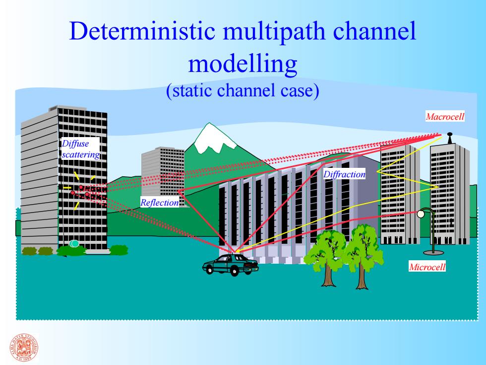
Deterministic multipath channel modelling (static channel case) Macrocell ■■■■■■ Diffuse scattering ■■■■ Diffraction ■■■ ■■■■ Reflection ■■■■■■ ■■ ■■ Microcell
Diffraction Microcell Macrocell Diffuse scattering Reflection Deterministic multipath channel modelling (static channel case)
Received signal with 1 path i-th ray 欧 ()白 x:=(0R.0R) 三 囟 RX Complex number representing the received signal(current) BelYR)gnl0z-0k R=-j π功 )-e时=pe (of course it is a funcion of the current I at the transmitter end) In particular we have: P amplitude Si,ti lenth,delay 8 phase % dicertion of arrival Doppler freq. 4 dicertion of departure
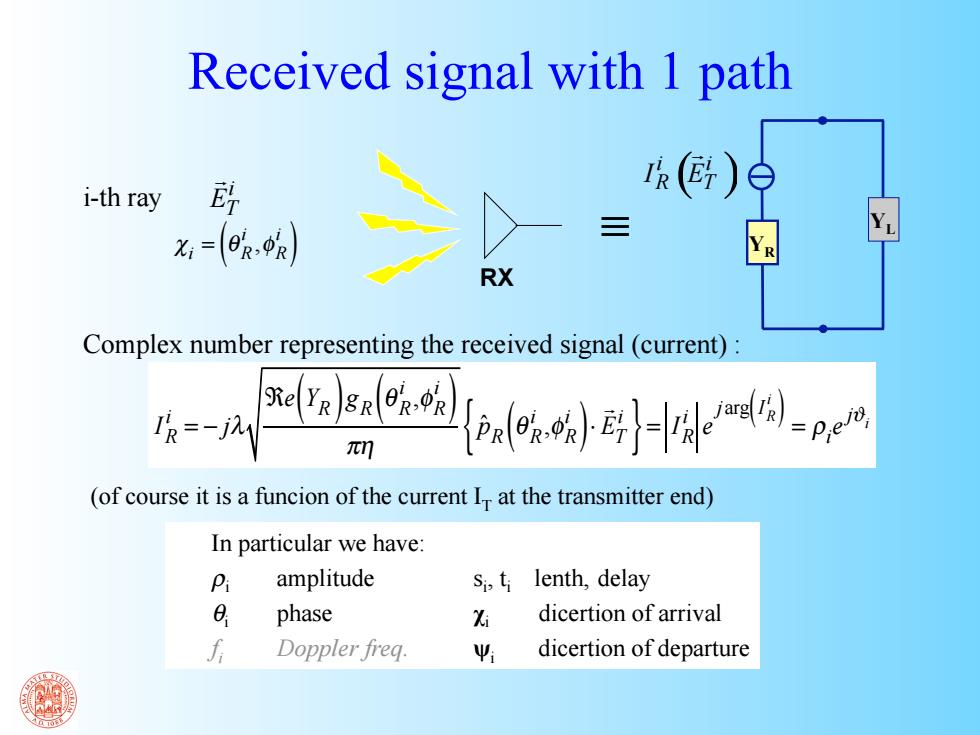
Received signal with 1 path IR i = − jλ ℜe Y( R ) gR θ R i ,φ R i ( ) πη pˆR θ R i ,φ R i ( )⋅ ET i { } = IR i e jarg IR i ( ) = ρi e jϑi RX i-th ray χi = θ R i ,φ R i ( ) ≡ In particular we have: ρi amplitude θi phase fi Doppler freq. si , ti lenth, delay χi dicertion of arrival ψi dicertion of departure Complex number representing the received signal (current) : (of course it is a funcion of the current IT at the transmitter end) i ET ( ) i i R T I E YR YL
Received signal with N.paths (1/2) -2-2pe四 In the narrowband case the new signal at the Rx is still a sinusoid,but with amplitude and phase given by the coherent sum(1).Time does not appear. In the wideband case,i.e.when a transmitted signal is modulated on the carrier we have to include the MO-DEM and consider the time domain Tx Rx u0中Mo x(t)Propagation channel Radio Channel_
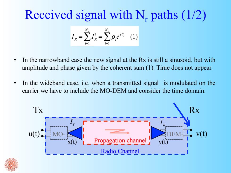
IR = IR i i=1 Nr ∑ = ρi e jϑi i=1 Nr ∑ (1) • In the narrowband case the new signal at the Rx is still a sinusoid, but with amplitude and phase given by the coherent sum (1). Time does not appear. • In the wideband case, i.e. when a transmitted signal is modulated on the carrier we have to include the MO-DEM and consider the time domain. Received signal with Nr paths (1/2) Tx Rx Radio Channel Propagation channel u(t) MO- DEM- v(t) x(t) y(t) IT IR
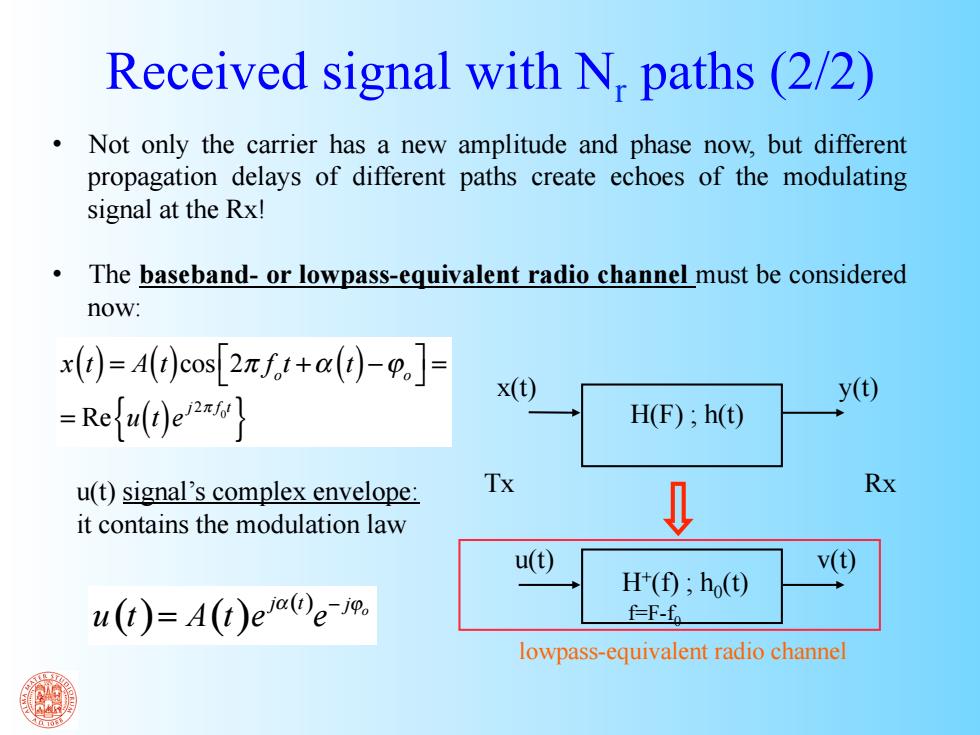
Received signal with N,paths(2/2) Not only the carrier has a new amplitude and phase now,but different propagation delays of different paths create echoes of the modulating signal at the Rx! The baseband-or lowpass-equivalent radio channel must be considered now: x(1)=A(t)cos[2zf.t+a()-0.J- x(t) -Refu(t)ex y(t) H(F);h(t) u(t)signal's complex envelope: Tx Rx it contains the modulation law u() v() H(0;h() u(t)=A(t)ee- f-F-fo lowpass-equivalent radio channel
x(t) y(t) H(F) ; h(t) u(t) v(t) H+(f) ; h0(t) f=F-f0 u(t) signal’s complex envelope: it contains the modulation law x(t) = A(t)cos 2π fo t +α (t) −ϕo ⎡ ⎣ ⎤ ⎦ = = Re u(t)e j2π f 0t { } ( ) ( ) ( ) o j t j u t A t e e α − ϕ = Received signal with Nr paths (2/2) • Not only the carrier has a new amplitude and phase now, but different propagation delays of different paths create echoes of the modulating signal at the Rx! • The baseband- or lowpass-equivalent radio channel must be considered now: Tx Rx lowpass-equivalent radio channel