Deterministic radio propagation modeling and ray tracing 1) Introduction to deterministic propagation modelling 2) Geometrical Theory of Propagation I-The ray concept-Reflection and transmission 3) Geometrical Theory of Propagation II-Diffraction,multipath 4) Ray Tracing I 5) Ray Tracing II-Diffuse scattering modelling 6) Deterministic channel modelling I 7) Deterministic channel modelling II-Examples 8) Project-discussion
1 Deterministic radio propagation modeling and ray tracing 1) Introduction to deterministic propagation modelling 2) Geometrical Theory of Propagation I - The ray concept – Reflection and transmission 3) Geometrical Theory of Propagation II - Diffraction, multipath 4) Ray Tracing I 5) Ray Tracing II – Diffuse scattering modelling 6) Deterministic channel modelling I 7) Deterministic channel modelling II – Examples 8) Project - discussion
Deterministic ray models (1/3) "Numerical simulation of multipath propagation according to GTP" Ray models compute(some of the)rays linking the two terminals through free space propagation and multiple interactions with buildings.The geometry and the field of such rays must satisfy GTP rules Interactions,i.e.reflections,diffractions,scatterings are also called "events" Usually all rays experiencing up to a pre-set number of events,N are computed .N also defines the so-called prediction order Ray models can be fully 3-Dimensional (3D)or can resort to simplified 2- dimensional modelling(2D) Ray models's output can be the field(before the Rx antenna)or the received signal (after the Rx antenna).In the latter case,Rx antenna parameters must be input to the model
Deterministic ray models (1/3) “Numerical simulation of multipath propagation according to GTP” • Ray models compute (some of the) rays linking the two terminals through free space propagation and multiple interactions with buildings. The geometry and the field of such rays must satisfy GTP rules • Interactions, i.e. reflections, diffractions, scatterings are also called “events”. Usually all rays experiencing up to a pre-set number of events, Nev are computed • Nev also defines the so-called prediction order • Ray models can be fully 3-Dimensional (3D) or can resort to simplified 2- dimensional modelling (2D) • Ray models’ s output can be the field (before the Rx antenna) or the received signal (after the Rx antenna). In the latter case, Rx antenna parameters must be input to the model. 2

Deterministic ray models (2/3) 。 Sometimes beams(tubes of flux)instead of"real"rays are considered.Rays have a null transverse dimension.Beams have a finite transverse dimension and therefore a space discretization is adopteda limit to space resolution is posed. Models adopting rays are usually referred to as Ray Tracing(RT)models. Models adopting beams are usually referred to as Ray (or beam)Launching(RL) models Ray models require in input a detailed description of the environment (environment database) Usually two different computation steps can be identified:geometric ray tracing and field computation.The former is by far the most CPU-time consuming Env.database geometric Field Results... Antenna data and other RT Comp. param. 3
Env. database geometric RT Field Comp. Results… • Sometimes beams (tubes of flux) instead of “real” rays are considered. Rays have a null transverse dimension. Beams have a finite transverse dimension and therefore a space discretization is adopted a limit to space resolution is posed. • Models adopting rays are usually referred to as Ray Tracing (RT) models. Models adopting beams are usually referred to as Ray (or beam) Launching (RL) models • Ray models require in input a detailed description of the environment (environment database) • Usually two different computation steps can be identified: geometric ray tracing and field computation. The former is by far the most CPU-time consuming Deterministic ray models (2/3) Antenna data and other param. 3
Deterministic ray models(3/3) Advantages over empirical-statistical models: Multipath simulation-multidimensional prediction High accuracy Great versatility Drawbacks: Environment database "cost" High CPU time (of the order of hours for urban prediction over a cell or area)
Multipath simulation → multidimensional prediction High accuracy Great versatility Environment database “cost” High CPU time (of the order of hours for urban prediction over a cell or area) Deterministic ray models (3/3) Advantages over empirical-statistical models: Drawbacks: 4
Performance Prediction accuracy first of all depends on the accuracy of environment database Prediction accuracy also depends on Nev:the greater Nev,the better the accuracy.Usually Nev=3-4 for outdoor,Nev=2 for indoor prediction are chosen. Unfortunately,CPU time grows more than linearly with Nv Prediction CPU time error 5
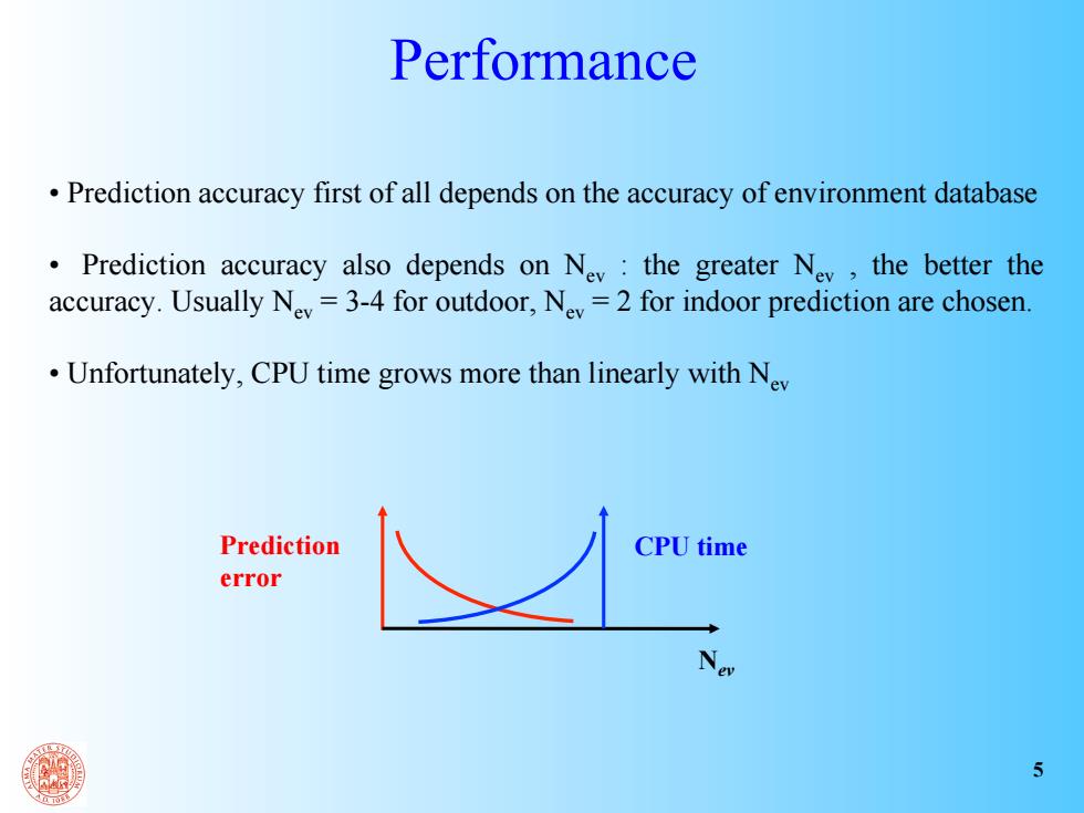
Nev Prediction error CPU time Performance • Prediction accuracy first of all depends on the accuracy of environment database • Prediction accuracy also depends on Nev : the greater Nev , the better the accuracy. Usually Nev = 3-4 for outdoor, Nev = 2 for indoor prediction are chosen. • Unfortunately, CPU time grows more than linearly with Nev 5