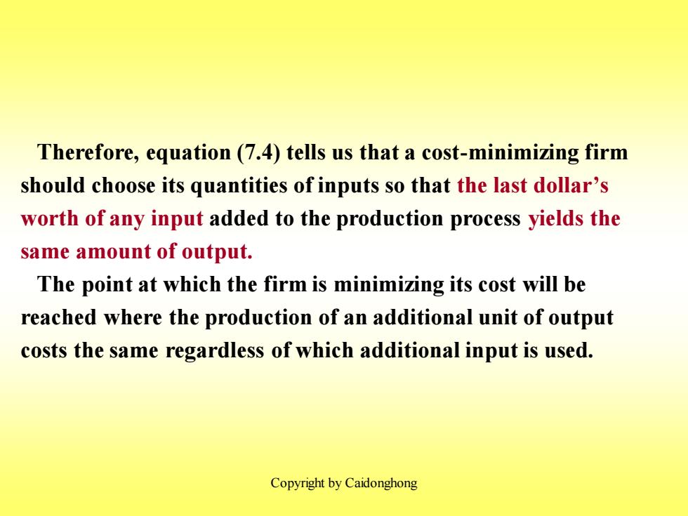
Therefore,equation (7.4)tells us that a cost-minimizing firm should choose its quantities of inputs so that the last dollar's worth of any input added to the production process yields the same amount of output. The point at which the firm is minimizing its cost will be reached where the production of an additional unit of output costs the same regardless of which additional input is used. Copyright by Caidonghong
Copyright by Caidonghong Therefore, equation (7.4) tells us that a cost-minimizing firm should choose its quantities of inputs so that the last dollar’s worth of any input added to the production process yields the same amount of output. The point at which the firm is minimizing its cost will be reached where the production of an additional unit of output costs the same regardless of which additional input is used
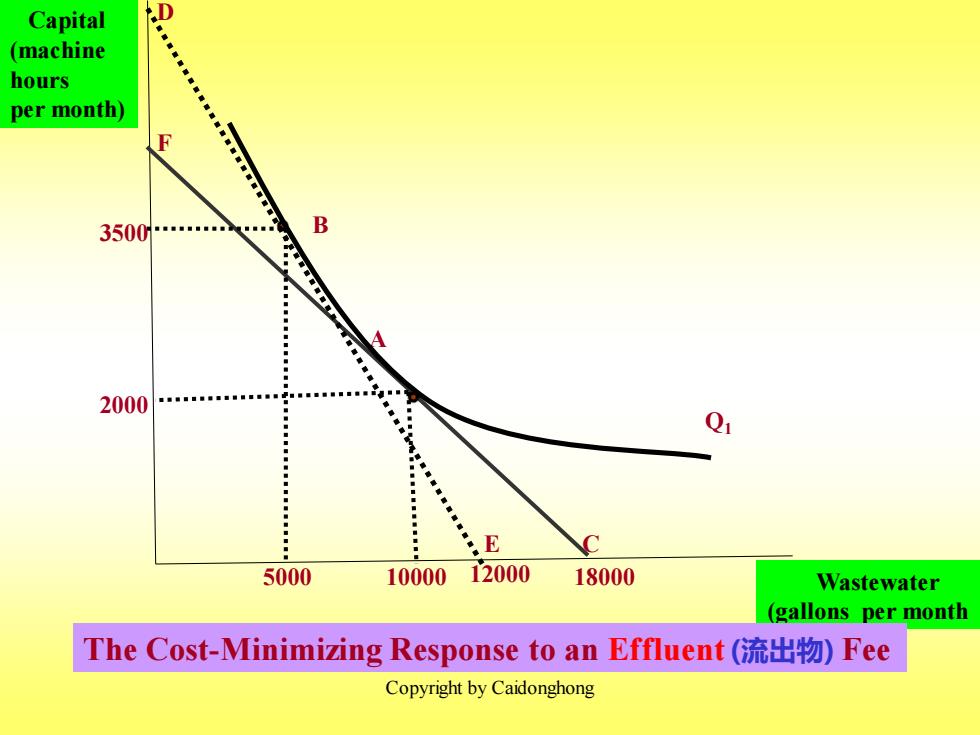
Capital D (machine hours per month) F 3500n B 2000 Q E 5000 1000012000 18000 Wastewater (gallons per month The Cost-.Minimizing Response to an Effluent(流出物)Fee Copyright by Caidonghong
Copyright by Caidonghong Q1 A Wastewater (gallons per month Capital (machine hours per month) 5000 E C 2000 3500 The Cost-Minimizing Response to an Effluent (流出物) Fee B 10000 12000 F D 18000

When the firm is not charged for dumping its wastewater in a river,it chooses to produce a given output using 10,000 gallons of wastewater and 2000 machine-hours of capital at A. However,an effluent fee raises the cost of wastewater,shifts the isocost curve from FC to DE,and causes the firm to produce at B-a process that results in much less effluent. Copyright by Caidonghong
Copyright by Caidonghong When the firm is not charged for dumping its wastewater in a river, it chooses to produce a given output using 10,000 gallons of wastewater and 2000 machine-hours of capital at A. However, an effluent fee raises the cost of wastewater, shifts the isocost curve from FC to DE, and causes the firm to produce at B-a process that results in much less effluent
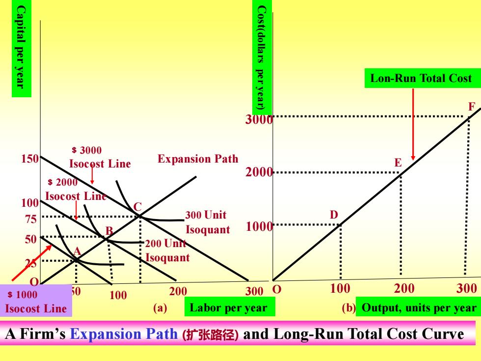
Capital per year Cost(dollars per year) Lon-Run Total Cost 3000 $3000 150 Isocost Line Expansion Path E 2000 $2000 100 Isocost Line 75 300 Unit 0 Isoquant 1000 50 200 Unn Isoquant $1000 50 100 200 3000 100 200 300 Isocost Line (a) Labor per year (b)Output,units per year A Firm's Expansion Path(扩张路径)and Long-Run Total Cost Curve
Copyright by Caidonghong Expansion Path A B C D E F 100 200 300 200 Unit Isoquant 300 Unit Isoquant 1000 2000 3000 100 200 300 ﹩2000 Isocost Line ﹩3000 Isocost Line 50 75 25 50 100 150 Capital per year (a) Labor per year (b) A Firm’s Expansion Path (扩张路径) and Long-Run Total Cost Curve ﹩1000 Isocost Line Cost(dollars per year) Lon-Run Total Cost Output, units per year O O
In(a),the expansion path(扩张路径)(from the origin through points A,B,and C)illustrates the least-cost combinations of labor and capital that can be used to produce each level of output in the long run-i.e.,when both inputs to production can be varied. In (b),the corresponding long-run total cost curve(from the origin through points D,E,and F)measures the least cost of producing the three output levels shown in (a). Copyright by Caidonghong
Copyright by Caidonghong In (a), the expansion path(扩张路径)(from the origin through points A, B, and C) illustrates the least-cost combinations of labor and capital that can be used to produce each level of output in the long run—i.e., when both inputs to production can be varied. In (b), the corresponding long-run total cost curve(from the origin through points D, E, and F)measures the least cost of producing the three output levels shown in (a)