
直方图 ni 当xeI,i=1,2,…,k 0, 其他 既是归一化参数,又表示每一组的组距,称为带宽或窗宽, Dissects the range of the data into bins of equal width along the horizontal axis Vertical axis represents the frequency counts(or percents,proportions)-Bars represent the counts Fewer bins,smoother histogram,but less detail about the distribution Trade-off between smoothness and detail:We want to preserve as much detail as possible but we do not want the graph to be too rough(difficult to discern shape)
直方图 • Dissects the range of the data into bins of equal width along the horizontal axis • Vertical axis represents the frequency counts (or percents, proportions)—Bars represent the counts • Fewer bins, smoother histogram, but less detail about the distribution • Trade-off between smoothness and detail: We want to preserve as much detail as possible but we do not want the graph to be too rough (difficult to discern shape)
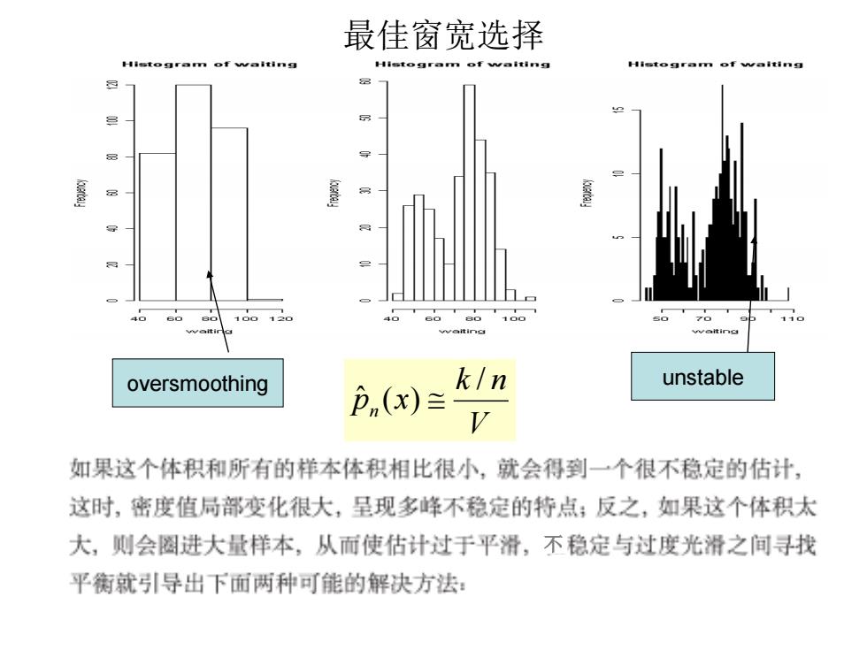
最佳窗宽选择 Histogram of waiting Histogram of weiting Histogram of walting 100120 100 11 waiting oversmoothing k/n unstable Pn(x) 如果这个体积和所有的样本体积相比很小,就会得到一个很不稳定的估计, 这时,密度值局部变化很大,呈现多峰不稳定的特点;反之,如果这个体积太 大,则会圈进大量样本,从而使估计过于平滑,不稳定与过度光滑之间寻找 平衡就引导出下而两种可能的解决方法:
V k n p x n / ˆ ( ) unstable oversmoothing 不 最佳窗宽选择
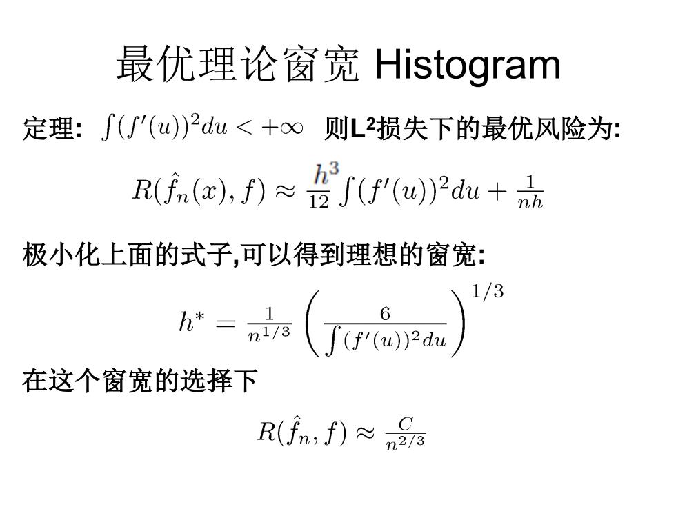
最优理论窗宽Histogram 定理:∫(∫'(u)2du<+o则L2损失下的最优风险为: rfn(x),f)≈jf'(u2a+ 极小化上面的式子,可以得到理想的窗宽: 1/3 =(Ta 在这个窗宽的选择下 R(f,f)≈nS
定理: 则L2损失下的最优风险为: 极小化上面的式子,可以得到理想的窗宽: 在这个窗宽的选择下 最优理论窗宽 Histogram
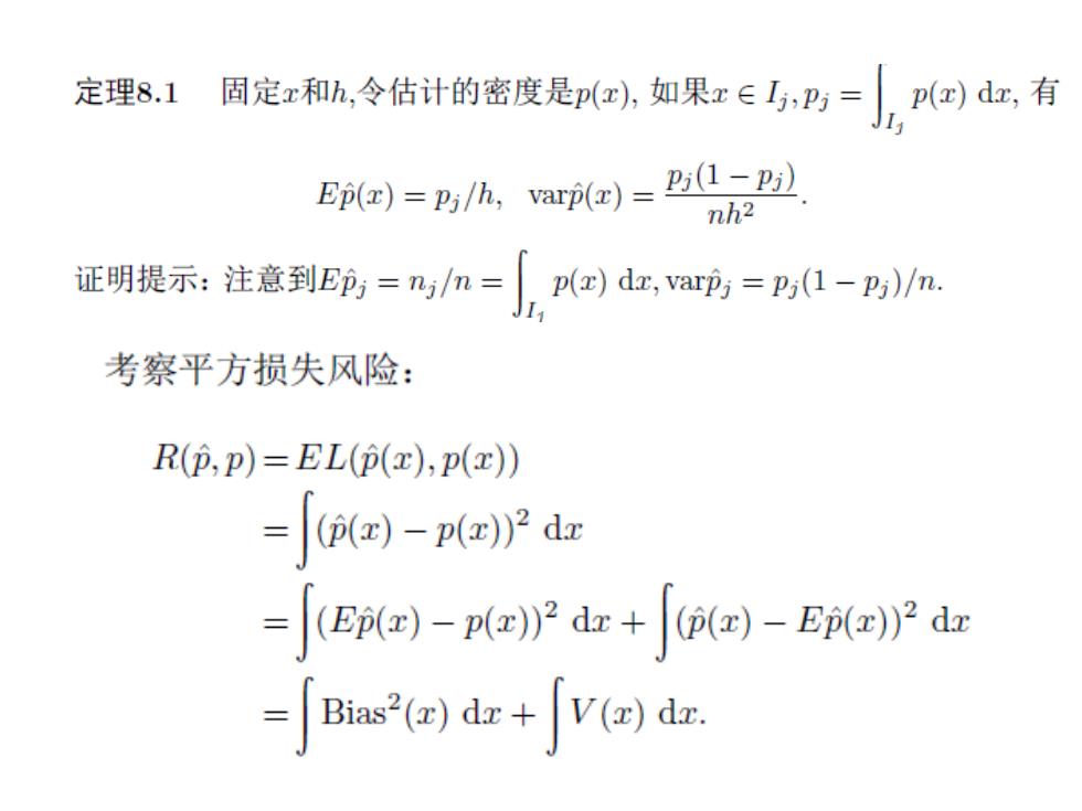
定理8.1 固定和h,令估计的密度是p,如果x∈马,=p)d,有 Ep(x)=Pi/h, apc)=P51-卫 nh2 证明提示:注意到E=nn= p()da,varpj pi(1-Pj)/n. 考察平方损失风险: R(p,p)=EL(p(x),p(x)) =(D(z)-p(z))2 dz -(Ep(=)-pz)dr+(p()-Epz))2 dzr =Bias()dr+v()回dk
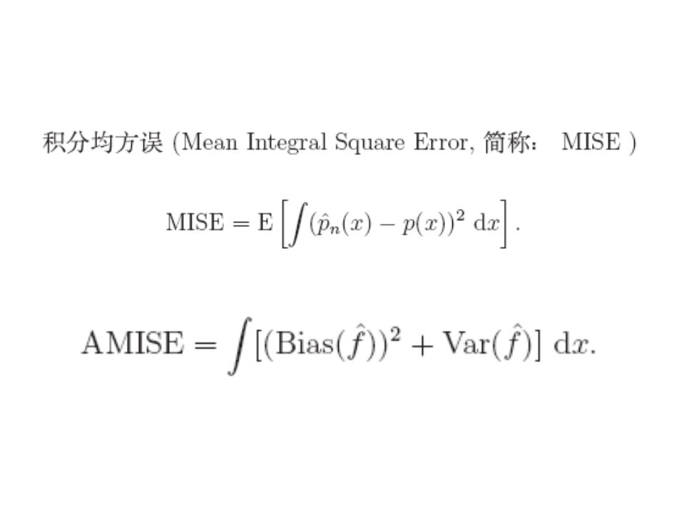
积分均方误(Mean Integral Square Error,简称:MISE) MISE-E(P(z)-p(z))2 dzr AMISE-[(Bias())+Var()dz