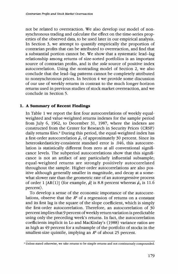
Contrarian Profits and Stock Market Overreaction not be related to overreaction.We also develop our model of non- synchronous trading and calculate the effect on the time-series prop- erties of the observed data,to be used later in our empirical analysis. In Section 3,we attempt to quantify empirically the proportion of contrarian profits that can be attributed to overreaction,and find that a substantial portion cannot be.We show that a systematic lead-lag relationship among returns of size-sorted portfolios is an important source of contrarian profits,and is the sole source of positive index autocorrelation.Using the nontrading model of Section 2,we also conclude that the lead-lag patterns cannot be completely attributed to nonsynchronous prices.In Section 4 we provide some discussion of our use of weekly returns in contrast to the much longer-horizon returns used in previous studies of stock market overreaction,and we conclude in Section 5. 1.A Summary of Recent Findings In Table 1 we report the first four autocorrelations of weekly equal- weighted and value-weighted returns indexes for the sample period from July 6,1962,to December 31,1987,where the indexes are constructed from the Center for Research in Security Prices (CRSP) daily returns files.During this period,the equal-weighted index has a first-order autocorrelation p,of approximately 30 percent.Since its heteroskedasticity-consistent standard error is .046,this autocorre- lation is statistically different from zero at all conventional signifi- cance levels.The subperiod autocorrelations show that this signifi- cance is not an artifact of any particularly influential subsample; equal-weighted returns are strongly positively autocorrelated throughout the sample.Higher-order autocorrelations are also pos- itive although generally smaller in magnitude,and decay at a some what slower rate than the geometric rate of an autoregressive process of order 1 [AR(1)](for example,p is 8.8 percent whereas p2 is 11.6 percent). To develop a sense of the economic importance of the autocorre- lations,observe that the R2 of a regression of returns on a constant and its first lag is the square of the slope coefficient,which is simply the first-order autocorrelation.Therefore,an autocorrelation of 30 percent implies that 9 percent of weekly return variation is predictable using only the preceding week's returns.In fact,the autocorrelation coefficients implicit in Lo and MacKinlay's (1988)variance ratios are as high as 49 percent for a subsample of the portfolio of stocks in the smallest-size quintile,implying an R2 of about 25 percent. Unless stated otherwise,we take returns to be simple returns and not continuously compounded. 179
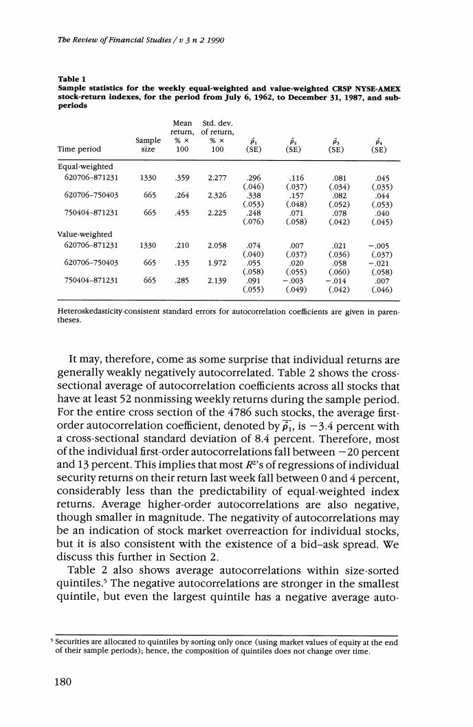
The Review of Financial Studies /v 3 n 2 1990 Table 1 Sample statistics for the weekly equal-weighted and value-weighted CRSP NYSE-AMEX stock-return indexes,for the period from July 6,1962,to December 31,1987,and sub- periods Mean Std.dev. return, of return, Sample %× %× P Time period size 100 100 (SE) (SE) (SE) (SE) Equal-weighted 620706-871231 1330 359 2.277 296 .116 .081 .045 (.046) (.037) (.034) (.035) 620706-750403 665 264 2.326 338 .157 .082 .044 (.053) (.048) (.052) (.053) 750404-871231 665 .455 2.225 ,248 .071 .078 .040 (.076) (.058) (.042) (.045) Value-weighted 620706-871231 1330 ,210 2.058 .074 .007 .021 -.005 (.040) (.037) (.036) (.037) 620706-750403 665 .135 1.972 .055 .020 .058 -.021 (.058) (.055) (.060) (.058) 750404-871231 665 ,285 2.139 .091 -.003 -.014 .007 (.055) (.049) (.042) (.046) Heteroskedasticity-consistent standard errors for autocorrelation coefficlents are given in paren- theses. It may,therefore,come as some surprise that individual returns are generally weakly negatively autocorrelated.Table 2 shows the cross- sectional average of autocorrelation coefficients across all stocks that have at least 52 nonmissing weekly returns during the sample period. For the entire cross section of the 4786 such stocks,the average first- order autocorrelation coefficient,denoted by p,is-3.4 percent with a cross-sectional standard deviation of 8.4 percent.Therefore,most of the individual first-order autocorrelations fall between-20 percent and 13 percent.This implies that most R2's of regressions of individual security returns on their return last week fall between 0 and 4 percent, considerably less than the predictability of equal-weighted index returns.Average higher-order autocorrelations are also negative, though smaller in magnitude.The negativity of autocorrelations may be an indication of stock market overreaction for individual stocks, but it is also consistent with the existence of a bid-ask spread.We discuss this further in Section 2. Table 2 also shows average autocorrelations within size-sorted quintiles.s The negative autocorrelations are stronger in the smallest quintile,but even the largest quintile has a negative average auto- s Securities are allocated to quintiles by sorting only once (using market values of equity at the end of their sample periods);hence,the composition of quintiles does not change over time. 180
Contrarian Profits and Stock Market Overreaction Table 2 Averages of autocorrelation coefficients for weekly returns on individual securities,for the period July 6,1962,to December 31,1987 Number of Sample securities (SD) (SD) 高 All stocks 4786 -.034 -,015 -.003 -.003 (.084) (.065) (.062) (.061) Smallest quintile 957 -.079 -.017 -.007 -.004 (.095) (.077) (.068) (.071) Central quintile 958 -,027 -.015 -.003 -,000 (.082) (.068) (.067) (,065) Largest quintile 957 -.013 -.014 -.002 -.005 (.054) (.050) (.050) (.047) The statistic p,is the average of th-order autocorrelation coefficients of returns on individual stocks that have at least 52 nonmissing returns.The population standard deviation (SD)is given in parentheses.Since the autocorrelation coefficients are not cross-sectionally independent,the re- ported standard deviations cannot be used to draw the usual inferences;they are presented merely as a measure of cross-sectional variation in the autocorrelation coefficients. correlation.Compared to the 30 percent autocorrelation of the equal- weighted index,the magnitudes of the individual autocorrelations indicated by the means (and standard deviations)in Table 2 are generally much smaller. To conserve space,we omit corresponding tables for daily and monthly returns,in which similar patterns are observed.Autocorre lations are strongly positive for index returns (35.5 and 14.8 percent p,'s for the equal-weighted daily and monthly indexes,respectively), and weakly negative for individual securities (-1.4 and-2.9 percent pI's for daily and monthly returns,respectively). The importance of cross-autocorrelations is foreshadowed by the general tendency for individual security returns to be negatively auto- correlated and for portfolio returns,such as those of the equal-and value-weighted market index,to be positively autocorrelated.To see this,observe that the first-order autocovariance of an equal-weighted index may be written as the sum of the first-order own-autocovariances and cross-autocovariances of the component securities.If the own- autocovariances are generally negative,and the index autocovariance is positive,then the cross-autocovariances must be positive. Moreover,the cross-autocovariances must be large,so large as to exceed the sum of the negative own-autocovariances.Whereas vir- tually all contrarian strategies have focused on exploiting the negative own-autocorrelations of individual securities [see,e.g.,DeBondt and Thaler (1985,1987)and Lehmann (1988)],primarily attributed to overreaction,we show below that forecastability across securities is at least as important a source of contrarian profits both in principle and in fact. .181
The Review of Financial Studies /v 3 n 2 1990 2.Analysis of Contrarian Profitability To show the relationship between contrarian profits and the cross effects that are apparent in the data,we examine the expected profits of one such strategy under various return-generating processes.Con- sider a collection of Nsecurities and denote by R,the N x 1 vector of their period t returns[R,···RwJ'.For convenience,we maintain the following assumption throughout this section: Assumption 1.R,is a jointly covariance-stationary stocbastic process with expectation ER,]=u=u,u2···4w'and autocovariance matrices E[(R-)(R-u)]=T wbere,with no loss ofgenerality, we take k=0 since =I.6 In the spirit of virtually all contrarian investment strategies,consider buying stocks at time t that were losers at time t-k and selling stocks at time t that were winners at time t-k,where winning and losing is determined with respect to the equal-weighted return on the market.More formally,if (k)denotes the fraction of the port- folio devoted to security i at time t,let w(k)=-(1/N0(Rm-k-Rnt-)i=1,..,N (1) where Rm=R/N is the equal-weighted market index.7 If, for example,k=1,then the portfolio strategy in period t is to short the winners and buy the losers of the previous period,t-1.By construction,w,(k)=[o(k)w2()···ωw()]'is an arbitrage port- folio since the weights sum to zero.Therefore,the total investment long (or short)at time t is given by I,(k)where lo(1 (2) Since the portfolio weights are proportional to the differences between the market index and the returns,securities that deviate more posi- tively from the market at time t-k will have greater negative weight 6Assumption 1 is made for notational simplicity,since joint covariance-stationarity allows us to eliminate time indexes from population moments such as and I;the qualitative features of our results will not change under the weaker assumptions of weakly dependent heterogeneously distributed vectors R.This would merely require replacing expectations with corresponding prob- ability limits of suitably defined time averages.The empirical results of Section 3 are based on these weaker assumptions;interested readers may refer to Assumptions A1-A3 in Appendix B. This is perhaps the simplest portfolio strategy that captures the essence of the contrarian principle. Lehmann (1988)also considers this strategy,although he employs a more complicated strategy in his empirical analysis in which the portfolio weights [Equation (1)]are renormalized each period by a random factor of proportionality,so that the investment is always $1 long and short.This portfolio strategy is also similar to that of DeBondt and Thaler (1985,1987),although in contrast to our use of weekly returns,they consider holding periods of three years.See Section 4 for further discussion. 182
Contrartan Profits and Stock Market Overreaction in the time t portfolio,and vice versa.Such a strategy is designed to take advantage of stock market overreactions as characterized,for example,by DeBondt and Thaler (1985):"(1)Extreme movements in stock prices will be followed by extreme movements in the oppo- site direction.(2)The more extreme the initial price movement,the greater will be the subsequent adjustment."The profit (k)from such a strategy is simply x,()=∑@()R。 (3) Rearranging Equation (3)and taking expectations yields the follow- ing: 肉1-g-点如)一片这a- (4) where um=E[Rm]=u'/N and tr()denotes the trace operator.8 The first term of Equation (4)is simply the kth-order autocovariance of the equal-weighted market index.The second term is the cross-sec- tional average of the kth-order autocovariances of the individual secu- rities,and the third term is the cross-sectional variance of the mean returns.Since this last term is independent of the autocovariances Ie and does not vary with k,we define the profitability indexL=L(T) and the constant o2(u)as (5) Thus, E[T,()]=L。-σ2(4) (6) For purposes that will become evident below,we rewrite L as Lw=C6十O (7) where G=1 KT4-tr(T] (8) Hence, π(k]=C+O。-σ2(u) (9) The derivation of Equation(4)is included in Appendix 1 for completeness.This is the population counterpart of Lehmann's (1988)sample moment equation (5)divided by N. 183