Review of Economic Studies (1991)58,529-546 0034-6527/91/00320529$02.00 C1991 The Review of Economic Studies Limited Speculative Dynamics DAVID M.CUTLER MIT JAMES M.POTERBA MIT and NBER and LAWRENCE H.SUMMERS Harvard University and NBER First version received January 1990;final version accepted February 1991 (Eds.) This paper presents evidence on the characteristic speculative dynamics of returns on stocks, bonds,foreign exchange,real estate,collectibles,and precious metals.It highlights four stylized facts.First,returns tend to be positively serially correlated at high frequency.Second,they are weakly negatively serially correlated over long horizons.Third,deviations of asset values from proxies for fundamental value have predictive power for returns.Fourth,short term interest rates are negatively correlated with excess returns on other assets.The similarity of the results across markets suggests that they may be due to inherent features of the speculative process Many recent studies have rejected the hypothesis of constant ex ante returns in a variety of different speculative markets.There is evidence that stock returns for the United States are weakly serially correlated,that dividend yields have predictive power for returns,that the slope of the yield curve predicts long-term bond returns,that interest rate spreads predict excess returns in the foreign exchange market,and more controversially,that asset markets display excess volatility.Research attempting to explain these findings has either challenged the statistical basis of rejections of the constant required return model, or sought to explain varying risk premia with changing risk factors. An alternative view is that variations in ex ante returns and asset market volatility arise primarily from what we have elsewhere labelled"speculative dynamics"-interac- tions between different types of traders,some of whom are not rational in the conventional sense of trading on the basis of all publicly available information.Distinguishing conclus- ively between the speculative dynamics view and the conventional view of asset market fluctuations is inherently very difficult,given the limited amount of data on asset returns and the difficulty of satisfactorily proxying for risk factors. This paper extends our research on speculative dynamics by introducing a larger and more diverse data set on speculative returns than has previously been analyzed. These data suggest four regularities in asset returns.First,asset returns are positively serially correlated at high frequencies.Second,returns are negatively serially correlated at lower frequencies.Third,there is a tendency toward"fundamental reversion"in asset prices.Finally,when short-term interest rates are high,the excess returns on other assets are low.Not all of these patterns emerge in all markets,but each appears in many different markets.Since risk factors might be expected to operate quite differently in different markets,we tentatively interpret the common patterns as evidence in favour of theories emphasizing speculative dynamics. 529 Copyright O 2001 All Rights Reserved

530 REVIEW OF ECONOMIC STUDIES This paper is organized as follows.Section one describes the data set covering asset returns in various markets.The second section reports the autocorrelogram of the various returns,emphasizing the similarities across markets.Section three discusses issues relating to fundamental reversion as well as the predictive power of short-term interest rates.The final section concludes by comparing the plausibility of the speculative dynamics and the time-varying returns interpretations of our results,and identifying directions for further research. 1.ASSET-RETURNS DATA This section describes the data we use in our subsequent analysis.Unlike past studies, which have relied almost exclusively on equity returns in the U.S.,our analysis includes returns in a wide range of asset markets.The data are available on diskette from the authors. Stocks and Bonds:Stock return data for the period 1960-1988 are drawn from Morgan Stanley's Capital International Perspectives (MSCI),augmented by data from Ibbotson Associates.For each of the thirteen equity markets in our sample--Australia, Austria,Belgium,Canada,France,Germany,Italy,Japan,Netherlands,Sweden,Switzer- land,United Kingdom,and United States-we calculate monthly excess returns R,.as R.=log (P..+D)-log (P..-1)-log (1+i) (1) where P.denotes the end-of-month price index for country j,D..dividend payments, and i,,the monthly short-term nominal interest rate.We chose these thirteen countries because they were the only ones in the Capital International universe with data back to 1960.The MSCI price index for each country is a weighted average of the prices for a number of large firms in the country's equity markets.These indices do not correspond to other published indices and often include shares traded on several different exchanges.? Our data on government bond returns are from Ibbotson Associates World Asser Module.Short-term yields are Treasury bill or money market yields,except in Italy, Sweden,and Switzerland,where we use the discount rate.The data sample for each country,for both bond and stock returns,is shown in Table 1.For comparability to earlier studies,we also report the results of autocorrelation tests applied to U.S.historical data from Ibbotson Associates (1988). Foreign Exchange:We compute the excess return to holding foreign currency assuming that investors making such investments hold foreign short-term bonds rather than cash.This implies that the excess return to a U.S.investor holding currency j is: Rts.=log (Eus./EUs..-1)+log (1+i )-log (1+ius.) (2) where the first term is the nominal appreciation of country i's currency relative to the dollar during month t.We focus on the returns to investors in each of five countries- France,Germany,Japan,the U.K.,and the U.S.-from holding the currencies of each of the other four countries.This yields 10 bilateral currency returns.Our sample period 1.MSCI computes dividend yields as aggregate dividends paid over the last twelve months divided by price at the end of the reference month.For several countries,dividend yields in the early part of the sample appear to reflect actual dividend payments rather than the sum of the previous year's payments.We adjusted these yields to make them comparable with the later sample.The resulting errors in the measured returns are likely to be smaller than those from omitting dividends altogether. 2.Poterba and Summers (1988)analyzed real (as distinct from excess)returns excluding dividends and computed from monthly averages of stock prices as reported by the International Monetary Fund. Copyright 2001 All Rights Reserved .....won
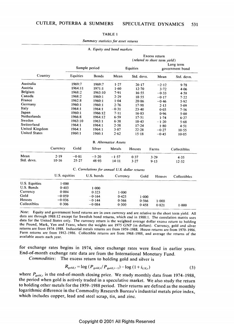
CUTLER,POTERBA SUMMERS SPECULATIVE DYNAMICS 531 TABLE 1 Summary statistics for asset returns A.Equity and bond markets Excess return related to short term yield) Long term Sample period Equities government bond Country Equities Bonds Mean Std.devn. Mean Std.devn. Australia 1969:7 1969:7 1-27 2617 -2.12 9-78 Austria 1964:11 1971:1 160 12.70 372 4-06 Belgium 1968:2 1963:10 791 16-55 -0-33 458 Canada 1968:2 1960:1 2·29 18-55 -017 722 France 1962:8 1960:1 1-04 20-86 -046 592 Germany 1960:1 1960:1 2.76 1798 213 5-09 Italy 1964:1 1964:1 -031 23.40 0-03 7.56 Japan 1960:1 1966:12 7,11 16-83 0-96 5-00 Netherlands 1966:8 1964:12 6-59 17-51 1.74 6·27 Sweden 1963:10 1963:1 6-38 18-43 1…20 568 Switzerland 1964:1 1964:1 2-58 17-24 1-80 451 United Kingdom 1964:1 1964:1 387 22-28 -0-27 1055 United States 1960:1 1960:1 262 15-18 -045 10-05 B.Alternative Assets Currency Gold Silver Metals Houses Farms Collectibles Mean 2-19 -081 -5·20 -157 037 3-29 435 Std.devn. 10-16 25-27 48-93 1411 327 9-13 12,32 C.Correlations for annual U.S.dollar returns U.S.equities U.S.bonds Currency Gold Houses Collectibles U.S.Equities 1-000 U.S.Bonds 0-403 1.000 Currency 0-004 0-323 1-000 Gold -0059 -0-164 0-425 1-000 Houses -0-036 -0-144 0566 0-566 1-000 Collectibles 0-306 -0084 0300 0:458 0-821 1-000 Note:Equity and government bond returns are in own currency and are relative to the short term yield.All data are through 1988:12 except for Swedish bond returns,which end in 1988:1.The correlation matrix uses data for the United States only.The currency return is the weighted average dollar excess return to holding the Pound,Mark,Yen and Franc,where the weights are 1975 GNP(in dollars).Currency,gold and silver returns are from 1974-1988.Industrial metals returns are from 1959-1988.House returns are from 1970-1986. Farm returns are from 1912-1986.Collectible returns are from 1968-1988,and average the returns of the available assets each year. for exchange rates begins in 1974,since exchange rates were fixed in earlier years. End-of-month exchange rate data are from the International Monetary Fund. Commodities:The excess return to holding gold and silver is Rgold.=log (Pgold./Pgold.-1)-log (1+ius.) (3) where Paold.,is the end-of-month closing price.We study monthly data from 1974-1988, the period when gold is actively traded in a speculative market.We also study the return to holding other metals for the 1959-1988 period.Their returns are defined as the monthly logarithmic difference in the Commodity Research Bureau's industrial metals price index, which includes copper,lead and steel scrap,tin,and zinc. Copyright 2001 All Rights Reserved

532 REVIEW OF ECONOMIC STUDIES Real Assets:We also analyze returns on houses and various collectibles.We measure excess holding returns under the assumption that these assets provide no service fow: R=l0g (P/P-1)-log (1+ius..). (4) Constant-quality house price indices are from Case and Shiller (1989).3 The data on collectibles,provided annually by Salomon Brothers for 1967-1988,cover oriental carpets, stamps,Chinese ceramics,rare books,coins,diamonds,and old master paintings. We also computed the return to holding farms by generalizing(4)to include a service flow term: Rfarm.=l0g Pfarm.!+Dfarm.)-log Pfarm.t-1)-log (1+ius.() (5) where Djarm.is aggregate farm income divided by aggregate farm value,then multiplied by the farm price index.The price is the average farm value per acre.Data on average value per are,1912-1986,were obtained from the Department of Agriculture (1981 and updates).Farm income data are from Colling and Irwin(1989). 2.AUTOCORRELATION OF ASSET RETURNS This section presents empirical evidence on the autocorrelation properties of asset returns. Analyzing many markets increases the statistical power of our tests,although in some cases the limited data span makes our findings relatively imprecise.The various markets should share any patterns that are common to the process of speculation,although risk considerations may differ across markets. Table I presents summary statistics on asset returns.The first panel focuses on equity and bond returns and shows substantial disparity in the mean returns across nations. Table 1 also shows the correlation between U.S.dollar returns on different classes of assets.The correlation between equity and bond returns is 0.403.The foreign exchange portfolio-a 1975 GNP-weighted average of the returns on the poind,franc,yen,and mark-exhibits a correlation of only 0-004 with U.S.equity returns,and its correlation with U.S.bond returns is 0.323.The real assets we analyze are highly correlated with each other,but negatively correlated with many other asset returns.Gold,houses and collectibles all exhibit cross-correlations of over 0.45,but the correlation between them and either stocks or bonds is small and usually negative.These findings suggest that our analysis of many different assets provides substantial evidence on the behaviour of speculative prices beyond that contained in equity returns. 2.1.The characteristic autocorrelogram of speculative returns Tables 2 through 4 present autocorrelograms for the various returns.We report the first order autocorrelation as well as the average autocorrelation over several distinct twelve month intervals.In each case,the reported autocorrelations have been corrected for small sample bias as described in the appendix. Table 2 presents the autocorrelations for stocks and bonds,Table 3 for foreign exchange and precious metals,and Table 4 for real assets.When we analyse data from 3.In order to avoid autocorrelation induced by measurement error,Case and Shiller formed an A and B price index for each city,using separate houses in each index.Our autocorrelations correlate contemporaneous values of the A series with lags of the B series.The results are very similar when the two series are reversed. www Copyright o 2001 All Rights Reserved

CUTLER,POTERBA SUMMERS SPECULATIVE DYNAMICS 533 TABLE 2 Autocorrelations for stock and bond returns Autocorrelations-excess returns relative to short-term treasury bills Months averaged in autocorrelations Asset 1-12 13-24 25-36 37-48 49-60 61-72 73-84 85-96 Corporate equities (1960-1988) Australia 0-028 0-002 -0-022 0-007 0012 0-003 -0-013 0-004 0-034 Austria 0-116 0-070 -0040 -0-002 -0007 -0-024 0-007 0-012 -0-014 Belgium 0-200 0-018 0006 0-040 0-009 0-016 -0022 0-033 -0-014 Canada 0-057 0-002 -0032 -0-004 0-G07 0-007 -0014 0-019 0039 France 0-083 0007 -0021 0-023 0-003 0-000 -0001 0-030 0-022 Germany 0-138 0-029 -0-042 0-002 0-006 -0-003 -0024 -0-003 0-044 Italy 0-138 0044 -0-040 0-000 -0017 0019 0-031 -0-013 0-031 Japan 0-085 0020 -0025 0019 0-004 -0-016 0-010 0-017 -0-013 Netherlands 0-114 0-021 -0015 0-004 0-010 0-002 -0-022 -0005 0-036 Sweden 0-134 0-038 -0041 0-022 0-001 0000 0-002 -0011 0-035 Switzerland 0046 0-017 -0019 -0-017 0-020 -0-007 -0019 0-008 0022 U.K. 0-091 0002 -0015 -0015 0011 0009 -0005 0-010 0-019 U.S. 0-077 -0-002 -0029 0004 0-017 0-019 -0016 0-000 0-041 Average 0-101 0021 -0-026 0-006 0-006 0-019 -0007 0-008 0-022 (0-030) (0-004) (0-0091 (0-006) (0-014) (0-016) (0-008) (0-011) (0-005) United States 0-106 0-021 -0-017 -0005 -0-011 -0006 0-000 0-012 0-013 (1926-1988) (0-036) (0011) (0011) (0-011) (0011) (0-011) (0011) (0-011) (0-011) Long-term bonds (1960-1988) Australia 0-078 0-036 -0-013 -0-032 -0-010 0012 0014 0022 0-008 Austria 0-360 0-119 -0-046 -0-067 -0003 0-013 -0-010 0-060 0-056 Belgium 0-191 0-110 0-006 -0-005 -0006 -0-023 -0-022 0-025 0012 Canada 0116 0-032 -0-008 -0-007 -0015 -0-020 0011 0-002 0-004 France 0230 0-086 -0-009 -0011 -0012 -0039 0-004 -0-003 0047 Germany 0477 0-106 -0-033 -0-041 -0-055 -0029 -0024 0003 0-051 Italy 0514 0-115 -0-003 -0-026 -0049 0018 -0018 0-078 -0010 Japan 0-132 0-062 -0-028 -0-036 -0-024 0024 0056 0-008 -0032 Netherlands 0291 0-043 -0-026 -0-017 -0015 0-013 -0-001 0-006 0023 Sweden 0-116 -0007 0-004 -0-006 -0015 0031 0-008 0-004 -0006 Switzerland 0-266 0-083 -0010 -0-045 -0-014 -0020 0-030 -0-012 0-010 U.K. 0-299 0-026 0-003 -0-039 -0014 0-031 0-036 0017 0-006 U.S. 0-030 0027 -0012 -0-005 0-008 -0-016 0-000 -0006 -0-003 Average 0-238 0-064 -0013 -0026 -0-017 -0-002 0-006 0-012 0013 (0-015) (0-004) (0-005) (0005) (0-005) (0005) (0-005) (0-005) (0-005) United States 0033 0023 -0-010 0-001 0-009 -0010 0-004 0-000 0-000 (1926-1988) (0036) (0011) (0011) (0-011) (0-011)(0-011)(0-011) (0011) (0-011) Note.Each entry reports the average autocorrelation for the 1 or 12 months in the indicated time period.The autocorrelations are bias-adjusted,by adding 1/(T-j)to each entry,where T is the length of the time period, andJ is the autocorrelation.The standard error of the individual correlations is (T-k)s,as in Kendall (1973).The standard error of the average autocorrelation,shown in parentheses,adjusts the predicted standard error for the cross-correlation of the assets,as indicated in the text. several countries,we also report the average autocorrelation at each frequency.We view this as a summary indication of the autocorrelation pattern,not as a deep parameter which characterizes behaviour in all markets.To indicate the precision of this average, we calculate its standard error assuming that the estimated statistics(such as the average of twelve autocorrelations)exhibit a constant pairwise correlation across countries, Copyright 2001 All Rights Reserved