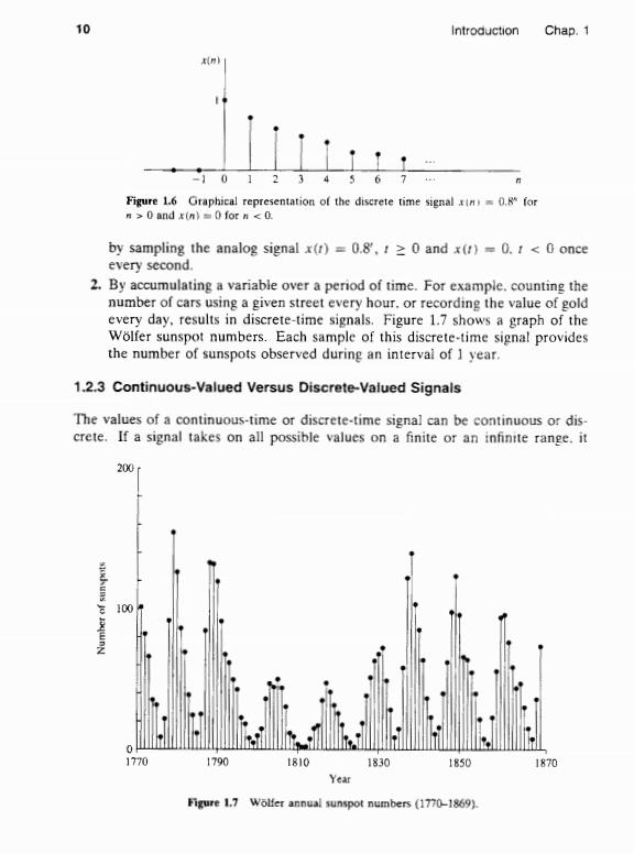
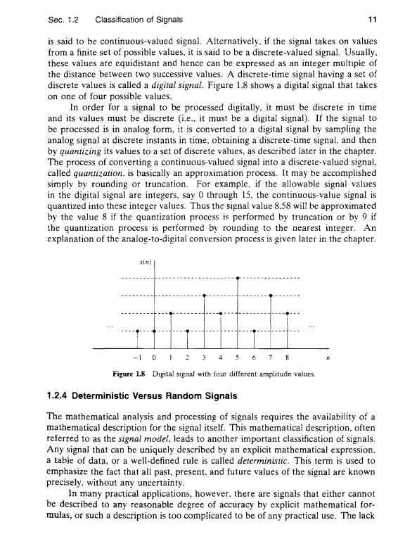
10 Introduction Chap.1 10123456 Figure 1.6 Graphical representation of the discrete time signal im 0.R for n>0 and (n)=0 for n <0. by sampling the analog signal x(t)=0.8',t0 and x(t)=0.t <0 once every second. 2.By accumulating a variable over a period of time.For example.counting the number of cars using a given street every hour.or recording the value of gold every day,results in discrete-time signals.Figure 1.7 shows a graph of the Wolfer sunspot numbers.Each sample of this discrete-time signal provides the number of sunspots observed during an interval of 1 year. 1.2.3 Continuous-Valued Versus Discrete-Valued Signals The values of a continuous-time or discrete-time signal can be continuous or dis- crete.If a signal takes on all possible values on a finite or an infinite range.it 200 00 0 1770 1790 t810 1830 1850 1870 Year Figure 1.7 Wolfer annual sunspot numbers (1770-1869)
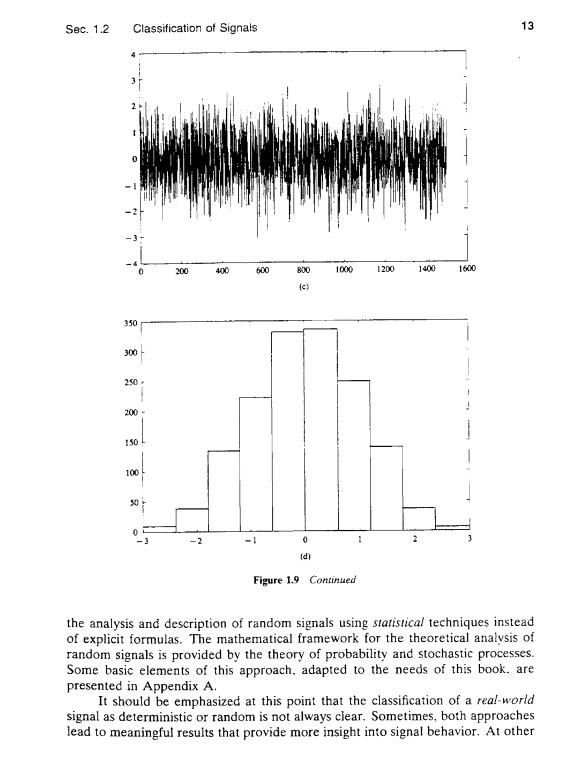
Sec.1.2 Classification of Signals 11 is said to be continuous-valued signal.Alternatively,if the signal takes on values from a finite set of possible values.it is said to be a discrete-valued signal.Usually, these values are equidistant and hence can be expressed as an integer multiple of the distance between two successive values.A discrete-time signal having a set of discrete values is called a digital signal.Figure 1.8 shows a digital signal that takes on one of four possible values. In order for a signal to be processed digitally,it must be discrete in time and its values must be discrete (i.e.,it must be a digital signal).If the signal to be processed is in analog form,it is converted to a digital signal by sampling the analog signal at discrete instants in time,obtaining a discrete-time signal,and then by quantizing its values to a set of discrete values.as described later in the chapter. The process of converting a continuous-valued signal into a discrete-valued signal, called quantization.is basically an approximation process.It may be accompiished simply by rounding or truncation.For example.if the allowable signal values in the digital signal are integers,say 0 through 15,the continuous-value signal is quantized into these integer values.Thus the signal value 8.58 will be approximated by the value 8 if the quantization process is performed by truncation or by 9 if the quantization process is performed by rounding to the nearest integer.An explanation of the analog-to-digital conversion process is given later in the chapter. 1n) -1012 3 46 78 Figure 18 Digital signal with four different amplitude values. 1.2.4 Deterministic Versus Random Signals The mathematical analysis and processing of signals requires the availability of a mathematical description for the signal itself.This mathematical description.often referred to as the signal model.leads to another important classification of signals. Any signal that can be uniquely described by an expiicit mathematical expression. a table of data,or a well-defined rule is called deterministic.This term is used to emphasize the fact that all past,present.and future values of the signal are known precisely,without any uncertainty. In many practical applications,however,there are signais that either cannot be described to any reasonable degree of accuracy by explicit mathematical for. mulas,or such a description is too complicated to be of any practical use.The lack

12 Introduction Chap.1 of such a relationship implies that such signals evolve in time in an unpredictable manner.We refer to these signals as random.The output of a noise generator, the seismic signal of Fig.1.4.and the speech signal in Fig.1.1 are examples of random signals. Figure 1.9 shows two signals obtained from the same noise generator and their associated histograms.Although the two signals do not resemble each other visually,their histograms reveal some similarities.This provides motivation for 200 400 600 8001000 1200 1400 1600 (a) 400 30: 300 250: 200 150 100- 0- 0 -3 -2 =1 0 2 6) Figure 1.9 Two random signals from the same signal gencrator and their his- tograms
S9c.1.2 Classification of Signals 13 200 400 600 800 1000 12001400 1600 (e) 350 300 20+ 200· 150L 100 0 0 d Figure 1.9 Continued the analysis and description of random signals using statistical techniques instead of explicit formulas.The mathematical framework for the theoretical analysis of random signals is provided by the theory of probability and stochastic processes. Some basic elements of this approach.adapted to the needs of this book.are presented in Appendix A. It should be emphasized at this point that the classification of a real-world signal as deterministic or random is not always clear.Sometimes,both approaches lead to meaningful results that provide more insight into signal behavior.At other
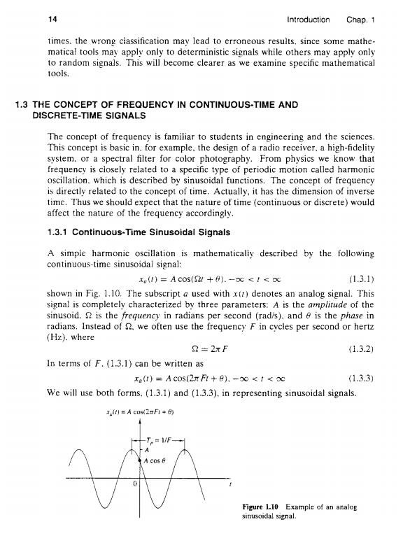
14 Introduction Chap.1 times.the wrong ciassification may lead to erroneous results.since some mathe- matical tools may apply only to deterministic signals while others may apply only to random signals.This will become clearer as we examine specific mathematical tools. 1.3 THE CONCEPT OF FREQUENCY IN CONTINUOUS-TIME AND DISCRETE-TIME SIGNALS The concept of frequency is familiar to students in engineering and the sciences. This concept is basic in.for example,the design of a radio receiver,a high-fidelity system.or a spectral filter for color photography.From physics we know that frequency is closely related to a specific type of periodic motion called harmonic oscillation.which is described by sinusoidal functions.The concept of frequency is directly related to the concept of time.Actually,it has the dimension of inverse time.Thus we should expect that the nature of time (continuous or discrete)would affect the nature of the frequency accordingly. 1.3.1 Continuous-Time Sinusoidal Signals A simpie harmonic oscillation is mathematically described by the following continuous-time sinusoidal signal: ()A cos(S2t +A).-oc<!<oc (1.3.1 shown in Fig.1.10.The subscript a used with x(r)denotes an analog signal.This signal is completely characterized by three parameters:A is the amplitude of the sinusoid.S is the frequency in radians per second (rad/s).and 6 is the phase in radians.Instead of S.we often use the frequency F in cycles per second or hertz (Hz).where 2=2πF (1.3.2) In terms of F.(1.3.1)can be written as xa(t)=A cos(2F+).-o<<oc (1.3.3) We will use both forms.(1.3.1)and (1.3.3).in representing sinusoidal signals. t)=A COs(2F1+0) Figure 1.10 Example of an analog sinusoidal signal