Outline (Level 2-3) 。Numeric Approach o Neural Network Terminologies Gradient Descent Principle o Stochastic Gradient Descent Algorithm 15/78
Outline (Level 2-3) Numeric Approach Neural Network Terminologies Gradient Descent Principle Stochastic Gradient Descent Algorithm 15 / 78
2.1.3.Stochastic Gradient Descent Algorithm for i=1to N W+1=W+n(d-wx)x' } It is called stochastic gradient descent(SGD) BGD algorithm is computationally intensive in the case of a relatively large training set. SGD algorithm oscillates around the minimum value,it can converge faster,and the algorithm can still be selected. 16/78
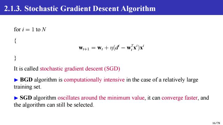
2.1.3. Stochastic Gradient Descent Algorithm for i = 1 to N { wt+1 = wt + η(d i − w T t x i )x i } It is called stochastic gradient descent (SGD) ▶ BGD algorithm is computationally intensive in the case of a relatively large training set. ▶ SGD algorithm oscillates around the minimum value, it can converge faster, and the algorithm can still be selected. 16 / 78
Outline (Level 2) ②Least Squares Method o Numeric Approach Analytic Approach 17/78
Outline (Level 2) 2 Least Squares Method Numeric Approach Analytic Approach 17 / 78
2.2.Analytic Approach Put all the training data together to form a large matrix. 「(x)I then∈RxM,X= 小e YE RNXM is design matrix or data matrix.Then get: w-dw-d=2∑Ixw-d=(w) 18/78
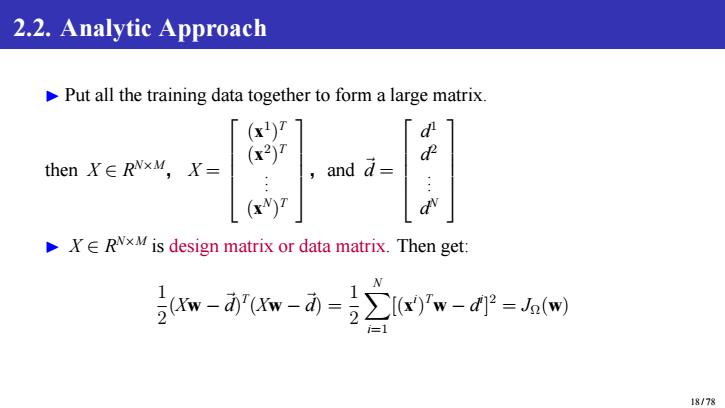
2.2. Analytic Approach ▶ Put all the training data together to form a large matrix. then X ∈ R N×M, X = (x 1 ) T (x 2 ) T . . . (x N ) T ,and ⃗d = d 1 d 2 . . . d N ▶ X ∈ R N×M is design matrix or data matrix. Then get: 1 2 (Xw −⃗d) T (Xw −⃗d) = 1 2 X N i=1 [(x i ) Tw − d i ] 2 = JΩ(w) 18 / 78
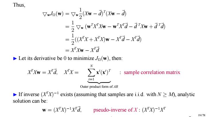
Thus, 7mwJn(w)=7.5w-aw-d =jVw(w'XXw-wXd-dxw+drd =j((Xx+XX)w-xq-xd) -XXw-Xd Let its derivative be 0 to minimize Jo(w),then: W XTXw-Xd,XX= x) sample correlation matrix i=1 Outer product form ofAB If inverse (XX)-1 exists (assuming that samples are i.i.d.with N>M),analytic solution can be: w=(xx-ra pseudo-inverse of Y:(XX)-1T 19/78
Thus, ▽wJΩ(w) = ▽w 1 2 (Xw −⃗d) T (Xw −⃗d) = 1 2 ▽w (w TX TXw − w TX T⃗d −⃗d TXw +⃗d T⃗d) = 1 2 ((X TX + X TX)w − X T⃗d − X T⃗d) = X TXw − X T⃗d ▶ Let its derivative be 0 to minimize JΩ(w), then: X TXw = X T⃗d, X TX = X N i=1 x i (x i ) T | {z } Outer product form of AB : sample correlation matrix ▶ If inverse (X TX) −1 exists (assuming that samples are i.i.d. with N ≥ M), analytic solution can be: w = (X TX) −1X T⃗d, pseudo-inverse of X : (X TX) −1X T X is formed by row vector form of feature vector x i , not column vector form. Therefore, X TX looks like a Gram Matrix, but actually not 19 / 78