Chapter 7:Multiscale Modeling of Composites 281 Application to a two-phase system When just one type of fiber is present,it follows from(7.28)and(7.29)that 吹公瓷 (7.30) The result(7.30)is now written in the form of the mixtures estimate plus a correction term as follows: h=4+G-匹-E (7.31) 以+Vn+吸 This result corresponds to one of the bounds derived using variational methods [1,2,10]and is identical to the result obtained when using the concentric cylinder model for a unidirectional,fiber-reinforced composite. 7.3.3 Transverse Shear It has been shown [8]that the effective transverse shear modulus for the multiphase composite is given by 24在引 (7.32) where 11 1 m (7.33) 121 Application to a two-phase system When just one type of fiber is present,it follows from(7.32)and (7.33)that 2+'k+1+')4k" A=听+2+0+0+2T (7.34) The result (7.34)is now written as a mixtures estimate plus a correction term so that
Application to a two-phase system When just one type of fiber is present, it follows from (7.28) and (7.29) that f m eff m f A mA A A f m mA f A (1 ) . (1 ) V V V V µ µ µ µ µ µ + + = + + (7.30) The result (7.30) is now written in the form of the mixtures estimate plus a correction term as follows: f m2 eff f m A A fm A f A mA m fm f A mA A ( ) . V V V V V V µ µ µ µµ µ µ µ − =+ − + + (7.31) This result corresponds to one of the bounds derived using variational methods [1, 2, 10] and is identical to the result obtained when using the concentric cylinder model for a unidirectional, fiber-reinforced composite. 7.3.3 Transverse Shear It has been shown [8] that the effective transverse shear modulus for the multiphase composite is given by eff m m m T TT T 1 11 12 , µ µµ 1 k ⎡ ⎛ ⎞⎤ = −Λ + ⎢ ⎜ ⎟⎥ + Λ ⎣ ⎝ ⎠⎦ (7.32) where m m eff TT TT f 1 m m m m eff TT T TT T 11 1 1 . 121 12 1 N i i i i V k k µµ µµ µ µµ µ = − − Λ ≡ = ++ ++ ∑ (7.33) Application to a two-phase system When just one type of fiber is present, it follows from (7.32) and (7.33) that f m mm f m eff m T T mT T f TT T T m m f m m m2 m T T T f TT f T 2 (1 ) . ( 2 ) (1 ) 2 ( ) Vk V k V k Vk V µµ µ µ µ µ µµ µ µ + ++ = + ++ + (7.34) The result (7.34) is now written as a mixtures estimate plus a correction term so that Chapter 7: Multiscale Modeling of Composites 281
282 L.N.McCartney 4=+4- (4-4)V (7.35) ++9 "+2 This result corresponds to one of the bounds derived using variational methods [1,2,10]. As results derived using Maxwell's methodology can correspond exactly to bounds obtained using variational methods,and to results obtained using the concentric cylinders model,it is clear that Maxwell's approach is not necessarily restricted to low fibre volume fractions where fibre interactions are negligible. To date,it has not been possible to find a method of using Maxwell's methodology to estimate the axial modulus and axial thermal expansion coefficient for a fiber-reinforced composite.However,the concentric cylinder model for a composite [6]leads to the following relations,which are expressed in the form of a mixtures estimate plus a correction term, EA=VEA+VER+ 4vs-v3-VV (7.36) 十 EAM aA =VEXCA+VEROR G+以ad-ag-吹a以.an + k味 The statement is now complete of all the analytical formulae that can be used to predict and completely characterize the thermoelastic properties of an undamaged unidirectional,fiber-reinforced composite.It only remains to state,in Sect.7.4,formulae for the extreme values that arise from variational calculations [1,2,10]and to provide conditions that determine whether the extreme values are upper or lower bounds. 7.4 Bounds for Composite Properties As already mentioned above,variational methods have been used [1,2,10] to estimate upper and lower bounds for the effective properties of both
f m2 eff f m T T fm T f T mT m m m f T T f T mT m m T T ( ) . 2 V V V V k V V k µ µ µ µµ µ µ µ µ − =+ − + + + (7.35) This result corresponds to one of the bounds derived using variational methods [1, 2, 10]. To date, it has not been possible to find a method of using Maxwell’s methodology to estimate the axial modulus and axial thermal expansion coefficient for a fiber-reinforced composite. However, the concentric cylinder model for a composite [6] leads to the following relations, which are expressed in the form of a mixtures estimate plus a correction term, f m2 eff f m A A A f A mA f m f m mf m TTT 4( ) , 1 E VE V E V V V V k k ν ν µ − =+ + + + (7.36) eff eff f f m m A A f AA mA A f m A A f f f m mm T AA T A A fm f m mf m TTT 4( ) [ ] . 1 E VE V E V V V V k k α αα ν ν α να α να µ = + − + + − − + + (7.37) The statement is now complete of all the analytical formulae that can be used to predict and completely characterize the thermoelastic properties of an undamaged unidirectional, fiber-reinforced composite. It only remains to state, in Sect. 7.4, formulae for the extreme values that arise from variational calculations [1, 2, 10] and to provide conditions that determine whether the extreme values are upper or lower bounds. 7.4 Bounds for Composite Properties As already mentioned above, variational methods have been used [1, 2, 10] to estimate upper and lower bounds for the effective properties of both L.N. McCartney As results derived using Maxwell’s methodology can correspond exactly to bounds obtained using variational methods, and to results obtained using the concentric cylinders model, it is clear that Maxwell’s approach is not necessarily restricted to low fibre volume fractions where fibre interactions are negligible. 282
Chapter 7:Multiscale Modeling of Composites 283 isotropic particulate and anisotropic fiber-reinforced composites.In many cases it is well known that the expressions for the bounds are such that interchanging fiber and matrix parameters merely interchanges the upper and lower bounds.One of the bounds corresponds to estimates that can be derived from spherical shell or concentric cylinder models,as described in [1].An examination of the literature regarding the conditions that determine the type of bound (either upper or lower)has revealed that there is a good deal of ambiguity.The objective of this section is to state the bounds for a particular property and to identify unambiguously the conditions that determine whether the extreme value of the property is an upper or lower bound.It should be noted that the required bounds are most easily derived by considering formulae for properties that have (as in Sect.7.3)been expressed as a mixtures estimate plus a correction term.It is easily seen that interchanging fiber and matrix parameters affects only one term in the denominator of the correction term.Many of the following conditions, determining the upper and lower bounds to be given,do not seem to appear in the literature.It should be noted that the correction terms all have a common structure involving proportionality to the product,orV and to the product of two reinforcement and matrix property differences,and that interchanging the reinforcement and matrix properties does not change the value of these products.It is emphasized that although the expressions given for the bounds differ in form to those that are quoted in [1,2,10],their values are in fact identical to the corresponding published expressions. 7.4.1 Bounds for Properties of Particulate Composites Bulk modulus Bounds for the bulk modulus of a particulate composite may be written in the following form ik。k (7.38) k V 3 k。 44m k 4μ where I V V (7.39)
7.4.1 Bounds for Properties of Particulate Composites Bulk modulus Bounds for the bulk modulus of a particulate composite may be written in the following form 2 2 p m p m p m p m m m p p eff pm m pm p 1 1 1 1 1 1 1 , 3 3 4 4 V V V V k k k k k k V V V V k k k µ µ k k ⎛⎞ ⎛⎞ ⎜⎟ ⎜⎟ − − ⎝⎠ ⎝⎠ − ≤ ≤ − + + + + (7.38) where p m p m 1 . V V kk k = + (7.39) Chapter 7: Multiscale Modeling of Composites isotropic particulate and anisotropic fiber-reinforced composites. In many cases it is well known that the expressions for the bounds are such that interchanging fiber and matrix parameters merely interchanges the upper and lower bounds. One of the bounds corresponds to estimates that can be derived from spherical shell or concentric cylinder models, as described in [1]. An examination of the literature regarding the conditions that determine the type of bound (either upper or lower) has revealed that there is a good deal of ambiguity. The objective of this section is to state the bounds for a particular property and to identify unambiguously the conditions that determine whether the extreme value of the property is an upper or lower bound. It should be noted that the required bounds are most easily derived by considering formulae for properties that have (as in Sect. 7.3) been expressed as a mixtures estimate plus a correction term. It is easily seen that interchanging fiber and matrix parameters affects only one term in the denominator of the correction term. Many of the following conditions, determining the upper and lower bounds to be given, do not seem to appear in the literature. It should be noted that the correction terms all have a common structure involving proportionality to the product, V Vp m or V Vf m , and to the product of two reinforcement and matrix property differences, and that interchanging the reinforcement and matrix properties does not change the value of these products. It is emphasized that although the expressions given for the bounds differ in form to those that are quoted in [1, 2, 10], their values are in fact identical to the corresponding published expressions. 283
284 L.N.McCartney These bounds are valid only if 4。≤lm, (7.40) and the bounds are reversed ifp Shear modulus Bounds for the shear modulus of a particulate composite may be written in the following form (4。-4m)2V'n π- ≤ler V,m+'m4,+ (9km +8um)um 6(km+24m) (7.41) (4。-4m)V'm Volm +Vmkp+ 9k。+8,), 6(k。+24,) where 正=V。+'mlm (7.42) These bounds are valid for the practically important case kp≥km,lp≥lm (7.43) and the bounds are reversed if kp≤km,lp≤lm Other cases can arise that are not considered here. Thermal expansion Bounds for the thermal expansion coefficient of a particulate composite may be written in the following form
p m µ ≤ µ , (7.40) and the bounds are reversed if µp ≥ µ m . Shear modulus Bounds for the shear modulus of a particulate composite may be written in the following form 2 p m pm eff m mm pm mp m m 2 p m pm p pp pm mp p p ( ) (9 8 ) 6( 2 ) ( ) , (9 8 ) 6( 2 ) V V k V V k V V k V V k µ µ µ µ µ µ µ µ µ µ µ µ µ µ µ µ µ − − ≤ + + + + − ≤ − + + + + where p p mm µ =V V µ µ + . (7.42) Thermal expansion Bounds for the thermal expansion coefficient of a particulate composite may be written in the following form L.N. McCartney These bounds are valid only if (7.41) p m p m k k ≥ , k k p m p m ≤ ≤ , . These bounds are valid for the practically important case and the bounds are reversed if Other cases can arise that are not considered here. ≥ µµ , (7.43) µ µ 284
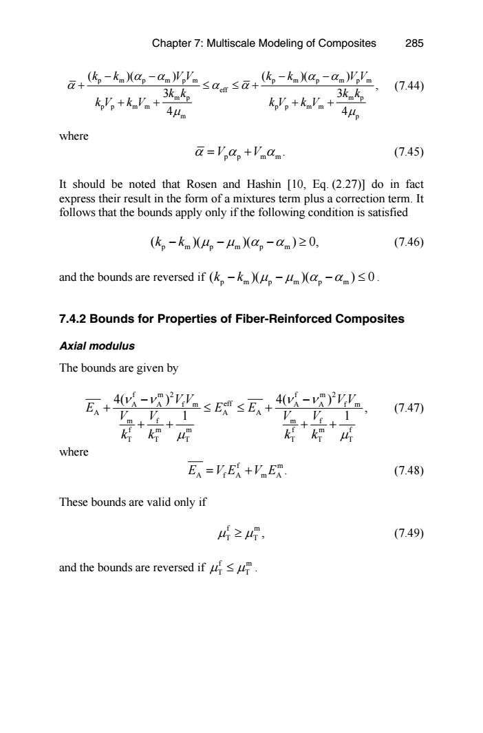
Chapter 7:Multiscale Modeling of Composites 285 g6,-kaX,-avsoah-kaXa,-ayV 3kmkp (7.44) k,'。+km'm+ 3kmkp 44m kolp+km!m+ 4μp where a='a。+Vnam (7.45) It should be noted that Rosen and Hashin [10,Eq.(2.27)]do in fact express their result in the form of a mixtures term plus a correction term.It follows that the bounds apply only if the following condition is satisfied (k。-km)4。-4m(a。-am)≥0, (7.46) and the bounds are reversed if(k,-km)(。-lm)(a。-am)≤0. 7.4.2 Bounds for Properties of Fiber-Reinforced Composites Axial modulus The bounds are given by Es+ -vW≤E≤E+ 4y-yΨ m++1 (7.47) m十 十 ” ki ki A where EA=VEA+VER (7.48) These bounds are valid only if ≥, (7.49) and the bounds are reversed ifusu
p m p m pm p m p m pm eff m p m p pp mm pp mm m p ( )( ) ( )( ) , 3 3 4 4 k k VV k k VV k k k k kV k V kV k V α α α α α α α µ µ − − − − + ≤ ≤ + + + + + (7.44) where p p mm α =V V α α + . (7.45) It should be noted that Rosen and Hashin [10, Eq. (2.27)] do in fact express their result in the form of a mixtures term plus a correction term. It follows that the bounds apply only if the following condition is satisfied pmp mp m ( )( )( ) 0, k k − − −≥ µ µαα (7.46) and the bounds are reversed if pmp mp m ( )( )( ) 0 k k − µ − −≤ µαα . 7.4.2 Bounds for Properties of Fiber-Reinforced Composites Axial modulus The bounds are given by f m2 f m2 A A fm eff A A fm A A A m f m f fmm fmf TT T TT T 4( ) 4( ) , 1 1 V V V V E E E V V V V k k k k ν ν ν ν µ µ − − + ≤ ≤ + + + + + (7.47) where f m A f A mA E VE V E = + . (7.48) These bounds are valid only if f m T T µ ≥ µ , (7.49) and the bounds are reversed if f m µ T T ≤ µ . Chapter 7: Multiscale Modeling of Composites 285