@月冷大学 Signal model for received signal In the case where L components are all specular path components,the output signal of the Rx antenna located at xRx while the Tx antenna located at Tx transmits signals can be written as L r(rTx,xRx;t)=∑aexp{i2x6'(De,Tx·ZTx)} = exp{2πλ'(e.Rx·xRx)} exp{2πvet}s(t-Te): (3) where s(t):the modulating signal at the input of the transmitter (Tx) antenna ■o:the wavelength. ae complex amplitude ■Te:delay SeRx:the incident direction eTx:the departure direction Graduate course:Propagatipn Channel Characterization,Parameter Estimation and Modeling 67/199
Signal model for received signal Graduate course: Propagation Channel Characterization, Parameter Estimation and Modeling 67 / 199 In the case where L components are all specular path components, the output signal of the Rx antenna located at xRx while the Tx antenna located at xTx transmits signals can be written as r ( xTx, xRx;t) = XL ℓ=1 α ℓ exp { j 2πλ − 1 0 ( Ωℓ,Tx · xTx ) } exp { j 2πλ − 1 0 ( Ωℓ,Rx · xRx ) } exp { j 2πνℓ t } s ( t − τℓ ). (3) where ■ s ( t ): the modulating signal at the input of the transmitter (Tx) antenna ■ λ 0 : the wavelength. ■ α ℓ : complex amplitude ■ τℓ : delay ■ Ωℓ,Rx : the incident direction ■ Ωℓ,Tx : the departure direction ■ νℓ : the Doppler frequency
@月命大凳 Direction of incidence characterized by T Direction (0,0,1) S2 sin(0) n 1cos(θ) 0,1,0 sin(0)cos() sin(e)sin(o) 1,0,0) Tx=e(Orx,Orx)=[cos(Orx)sin(OTx),sin(orx)sin(Orx),cos(0Tx)]TES2 Graduate course:Propagation Channel Characterization,Parameter Estimation and Modeling 68/199
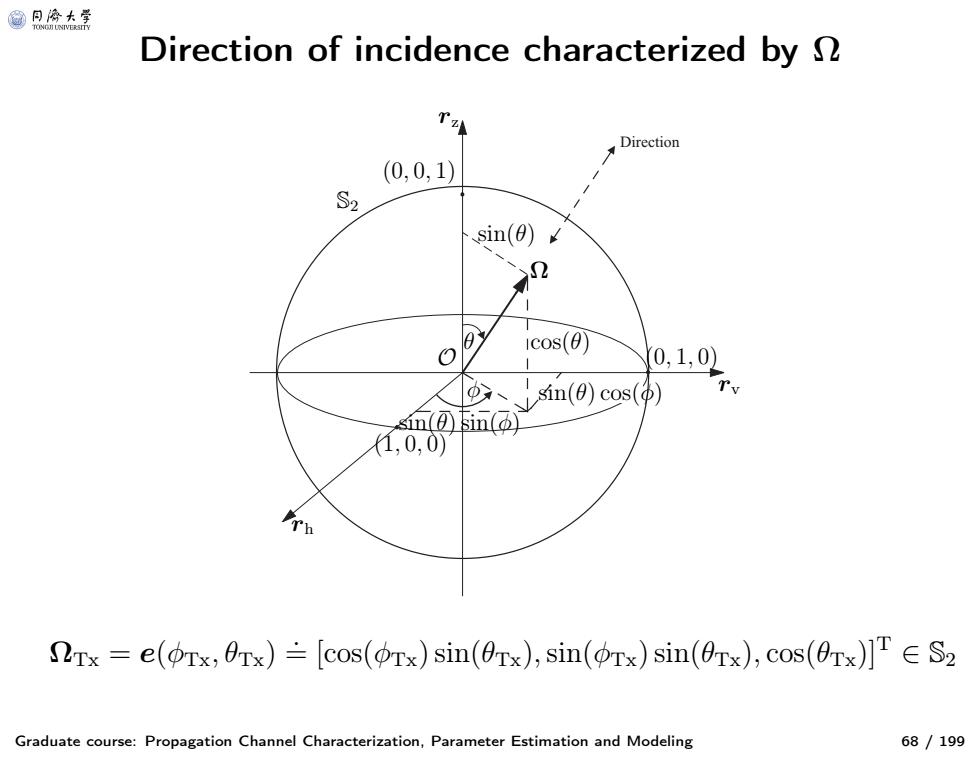
Direction of incidence characterized by Ω Graduate course: Propagation Channel Characterization, Parameter Estimation and Modeling 68 / 199 Direction S 2 r h r v r z (0, 0, 1) (0, 1, 0) (1, 0, 0) sin( θ) cos( θ) sin( θ) sin( φ) sin( θ) cos( φ) θ φ O Ω ΩTx = e ( φTx, θTx ) .= [cos( φTx) sin( θTx ),sin( φTx) sin( θTx ), cos( θTx)] T ∈ S 2
@月傍大学 Bidirection-delay-Doppler spread function r,0=/∫∫∫exp2xA'nxn} exp{j2mXo(SRx Rx)}exp{j2mvt}s(t-T) h(STx,SRx,T,v)dsTxdsRxdrdv. (4) where h(2rx,2Rx,T,))=∑ad(2rx-2rx)i(2Rx-2Rxe) =1 δ(T-Te)6(v-v). (5) is called spread function. Graduate course:Propagation Channel Characterization,Parameter Estimation and Modeling 69/199
Bidirection-delay-Doppler spread function Graduate course: Propagation Channel Characterization, Parameter Estimation and Modeling 69 / 199 r ( xTx, xRx;t) = Z Z Z Z exp { j 2πλ − 1 0 ( ΩTx · xTx ) } exp { j 2πλ − 1 0 ( ΩRx · xRx ) } exp { j 2πνt } s ( t − τ ) h ( ΩTx, ΩRx, τ, ν)d ΩTx d ΩRx d τ dν. (4) where h ( ΩTx, ΩRx, τ, ν) = XL ℓ=1 α ℓ δ ( ΩTx − ΩTx,ℓ ) δ ( ΩRx − ΩRx,ℓ ) δ ( τ − τℓ ) δ ( ν − νℓ ). (5) is called spread function
@凡冷大学 Property of the spread function The expectation of the spread function is 0,i.e. E[h(2Tx,2Rx,T,v)]=0. (6) Under the US assumption: E[h(STx,SRx;T;v)h(Sx;SRx T,V)=P(STx,SRx:T,v) 6(2mx-nx)6(2Rx-2Rx)6(T-T)6(w-V) (7) where P(Tx,2Rx,T,v)=E[lh(2Tx,2Rx,T,v)川2] (8) is called the bidirection-delay-Doppler power spectrum Graduate course:Propagation Channel Characterization,Parameter Estimation and Modeling 70/199
Property of the spread function Graduate course: Propagation Channel Characterization, Parameter Estimation and Modeling 70 / 199 The expectation of the spread function is 0, i.e. E[ h ( ΩTx, ΩRx, τ, ν)] = 0. (6) Under the US assumption: E[ h ( ΩTx,ΩRx, τ, ν ) h ( Ω ′ Tx , Ω ′ Rx, τ ′, ν ′)] = P ( ΩTx, ΩRx, τ, ν ) δ ( ΩTx − Ω ′ Tx ) δ ( ΩRx − Ω ′ Rx ) δ ( τ − τ ′ ) δ ( ν − ν ′ ) (7) where P ( ΩTx, ΩRx, τ, ν) = E[|h ( ΩTx, ΩRx, τ, ν )| 2 ] (8) is called the bidirection-delay-Doppler power spectrum
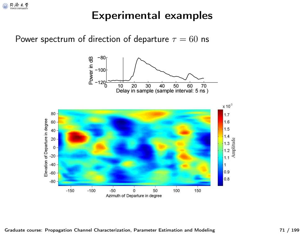
@月冷大等 Experimental examples Power spectrum of direction of departure T=60 ns -80 -100 10203040506070 Delay in sample(sample interval:5 ns 10 1.7 15 1211 09 80 .150 -100 50 0 50 100 150 Azimuth of Departure in degree Graduate course:Propagation Channel Characterization,Parameter Estimation and Modeling 71/199
Experimental examples Graduate course: Propagation Channel Characterization, Parameter Estimation and Modeling 71 / 199 Power spectrum of direction of departure τ = 60 ns 0 10 20 30 40 50 60 70 −120 −100 −80 Delay in sample (sample interval: 5 ns ) Power in dB