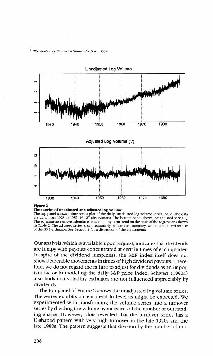
Tbe Review of Financial Studies/v5n 2 1992 Unadjusted Log Volume 1930 1940 1950 1960 1970 1980 Adjusted Log Volume(v) 1930 1940 1950 1960 1970 1980 Figure 2 Time series of unadjusted and adjusted log volume The top panel shows a time-series plot of the daily unadjusted log volume series log V.The data are daily from 1928 to 1987,16,127 observations.The bottom panel shows the adjusted series v The adjustments remove calendar effects and long-term trend on the basis of the regressions shown in Table 2.The adjusted series v,can reasonably be taken as stationary,which is required for use of the SNP estimator.See Section 1 for a discussion of the adjustments. Our analysis,which is available upon request,indicates that dividends are lumpy with payouts concentrated at certain times of each quarter. In spite of the dividend lumpiness,the S&P index itself does not show detectable movements in times of high dividend payouts.There- fore,we do not regard the failure to adjust for dividends as an impor- tant factor in modeling the daily S&P price index.Schwert (1990a) also finds that volatility estimates are not influenced appreciably by dividends. The top panel of Figure 2 shows the unadjusted log volume series. The series exhibits a clear trend in level as might be expected.We experimented with transforming the volume series into a turnover series by dividing the volume by measures of the number of outstand- ing shares.However,plots revealed that the turnover series has a U-shaped pattern with very high turnover in the late 1920s and the late 1980s.The pattern suggests that division by the number of out- 208
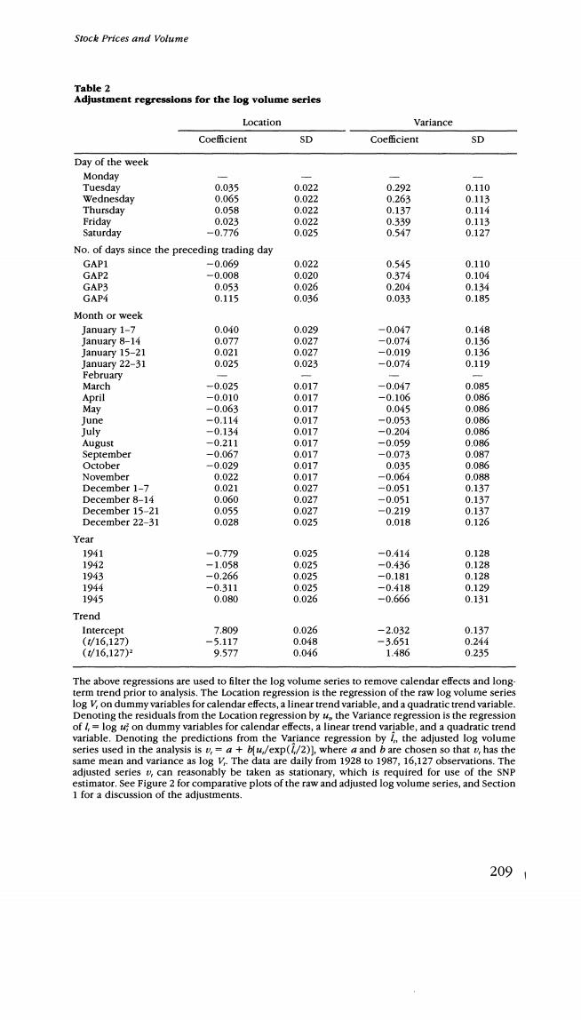
Stock Prices and Volume Table 2 Adjustment regressions for the log volume series Location Variance Coefficient SD Coefficient SD Day of the week Monday Tuesday 0.035 0.022 0.292 0.110 Wednesday 0.065 0.022 0.263 0.113 Thursday 0.058 0.022 0.137 0.114 Friday 0.023 0.022 0.339 0.113 Saturday -0.776 0.025 0.547 0.127 No.of days since the preceding trading day GAP1 -0.069 0.022 0.545 0.110 GAP2 -0.008 0.020 0.374 0.104 GAP3 0.053 0.026 0.204 0.134 GAP4 0.115 0.036 0.033 0.185 Month or week January 1-7 0.040 0.029 -0.047 0.148 January 8-14 0.077 0.027 一0.074 0.136 January 15-21 0.021 0.027 -0.019 0.136 January 22-31 0.025 0.023 -0.074 0.119 February March -0.025 0.017 -0.047 0.085 April -0.010 0.017 -0.106 0.086 Mav -0.063 0.017 0.045 0.086 June -0.114 0.017 -0.053 0.086 July -0.134 0.017 -0.204 0.086 August -0.211 0.017 -0.059 0.086 September -0.067 0.017 -0.073 0.087 October -0.029 0.017 0.035 0.086 November 0.022 0.017 -0.064 0.088 December 1-7 0.021 0.027 -0.051 0.137 December 8-14 0.060 0.027 -0.051 0.137 December 15-21 0.055 0.027 -0.219 0.137 December 22-31 0.028 0.025 0.018 0.126 Year 1941 -0.779 0.025 -0.414 0.128 1942 -1.058 0.025 -0.436 0.128 1943 -0.266 0.025 -0.181 0128 1944 -0.311 0.025 -0413 0.129 1945 0.080 0.026 -0.666 0.131 Trend Intercept 7.809 0.026 -2.032 0.137 (t/16,127) -5.117 0.048 -3.651 0.244 (16.127) 9.577 0.046 1.486 0.235 The above regressions are used to filter the log volume series to remove calendar effects and long term trend prior to analysis.The Location regression is the regression of the raw log volume series log V,on dummy variables for calendar effects,a linear trend variable,and a quadratic trend variable. Denoting the residuals from the Location regression by t the Variance regression is the regression of /log t on dummy variables for calendar effects,a linear trend variable,and a quadratic trend variable.Denoting the predictions from the Variance regression by the adjusted log volume series used in the analysis is v,=a +bfu/exp(/2)],where a and b are chosen so that v,has the same mean and variance as log V.The data are daily from 1928 to 1987,16,127 observations.The adjusted series v,can reasonably be taken as stationary,which is required for use of the SNP estimator.See Figure 2 for comparative plots of the raw and adjusted log volume series,and Section 1 for a discussion of the adjustments. 2091
Tbe Review of Financial Studies/v5n 2 1992 standing shares is an inadequate detrending strategy.Thus,we decided to include a quadratic trend in both the mean and variance equation for volume along with the same dummy variables to account for cal- endar and wartime effects as were used in adjusting the price change series.As seen from Table 2,volume is lower on Monday and Saturday, and there are pronounced seasonal patterns by month of the year, with lower volume in the summer months.In all but the last of the war years,the level of volume was much lower than normal.The adjusted log volume series shown in the bottom panel of Figure 2 shows relatively homogeneous variation around a mean level. It is important to note that our quadratic detrending of price vol- atility and the volume series is best viewed as a band limited filter that passes everything except extremely low-frequency behavior.We certainly do not suggest that these trends can be extrapolated.Officer (1973)and Schwert(1989)conclude that great depression is simply an unusual event with two to three times higher volatility than any other period since 1870.Schwert(1990b)suggests that the crash of 1987 is also characterized by unusually high volatility.An alternative to detrending would be to introduce dummy variables for the depres- sion and the 1987 crash period.But evidence in the data that there has been a gradual increase in volatility since the early 1970s per- suaded us that a U-shaped quadratic trend is a more reasonable pro- cedure. The adjustment procedures are designed to remove long-run trend and those systematic calendar effects that are well documented.We have taken care to make adjustments only for effects for which there is statistical evidence in Tables 1 and 2,or for which there is evidence in the previous work cited above.Figures 1 and 2 summarize the adjustments and suggest that they do,in fact,make the series more amenable to analysis with a stationary time-series model. Note that the procedures treat the price change and volume vari- ables in essentially the same way.Thus,inferences based on fitting the dynamics of adjusted data will be very close to inferences that would be obtained from fitting unadjusted data,but with parameters on calendar dummies estimated jointly with everything else.In the case of linear models,inferences would be exactly the same;in the nonlinear case,the equivalence is only approximate.In view of the scale of models required to characterize the nonlinear process,it is computationally intractable to undertake such joint estimation,and our two-step procedure is a computational compromise. Appropriate procedures for handling regular calendar variation in data have long been debated in the seasonality literature,which has yet to come to a consensus.Recently,Sims (1991)and Hansen and Sargent (1991)present strong cases for making seasonality adjust- 210
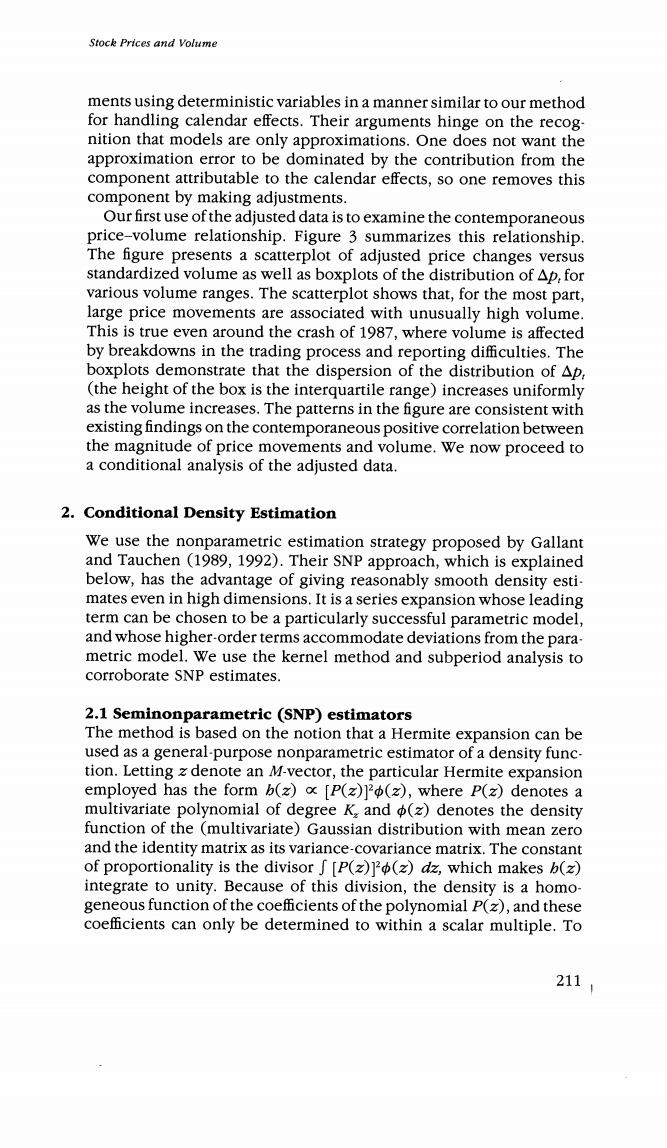
Stock Prices and Volume ments using deterministic variables in a manner similar to our method for handling calendar effects.Their arguments hinge on the recog- nition that models are only approximations.One does not want the approximation error to be dominated by the contribution from the component attributable to the calendar effects,so one removes this component by making adjustments. Our first use of the adjusted data is to examine the contemporaneous price-volume relationship.Figure 3 summarizes this relationship. The figure presents a scatterplot of adjusted price changes versus standardized volume as well as boxplots of the distribution of Ap,for various volume ranges.The scatterplot shows that,for the most part, large price movements are associated with unusually high volume. This is true even around the crash of 1987,where volume is affected by breakdowns in the trading process and reporting difficulties.The boxplots demonstrate that the dispersion of the distribution of Ap, (the height of the box is the interquartile range)increases uniformly as the volume increases.The patterns in the figure are consistent with existing findings on the contemporaneous positive correlation between the magnitude of price movements and volume.We now proceed to a conditional analysis of the adjusted data. 2.Conditional Density Estimation We use the nonparametric estimation strategy proposed by Gallant and Tauchen (1989,1992).Their SNP approach,which is explained below,has the advantage of giving reasonably smooth density esti- mates even in high dimensions.It is a series expansion whose leading term can be chosen to be a particularly successful parametric model, and whose higher-order terms accommodate deviations from the para- metric model.We use the kernel method and subperiod analysis to corroborate SNP estimates. 2.1 Seminonparametric (SNP)estimators The method is based on the notion that a Hermite expansion can be used as a general-purpose nonparametric estimator of a density func- tion.Letting z denote an M-vector,the particular Hermite expansion employed has the form b(z)[P(z)2(z),where P(z)denotes a multivariate polynomial of degree K and (z)denotes the density function of the (multivariate)Gaussian distribution with mean zero and the identity matrix as its variance-covariance matrix.The constant of proportionality is the divisor f [P(z)(z)dz,which makes b(z) integrate to unity.Because of this division,the density is a homo- geneous function of the coefficients of the polynomial p(z),and these coefficients can only be determined to within a scalar multiple.To 211
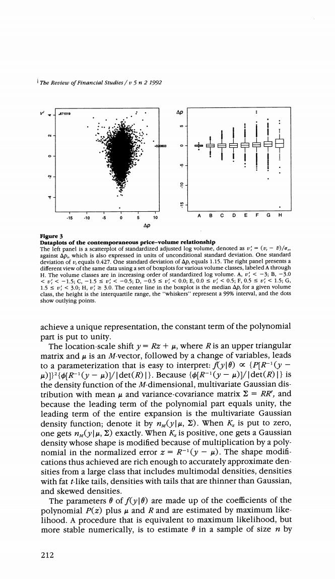
The Review of Financial Studies /v 5 n 2 1992 871019 *宁宁学中中的 A -15 B C D E F G H .10 0 Figure 3 Dataplots of the contemporaneous price-volume relationship The left panel is a scatterplot of standardized adjusted log volume,denoted as v=(v,-)/ against Ap,,which is also expressed in units of unconditional standard deviation.One standard deviation of vequals 0.427.One standard deviation of Ap,equals 1.15.The right panel presents a different view of the same data using a set of boxplots for various volume classes,labeled A through H.The volume classes are in increasing order of standardized log volume.A,v<-3;B,-3.0 <vf<-1.5:C,-1.5≤<-0.5:D,-0.5≤<0.05E,0.0≤:<05;E,0.5s(<1.5:G 1.5s<3.0;H,v2 3.0.The center line in the boxplot is the median Ap,for a given volume class,the height is the interquartile range,the"whiskers"represent a 99%interval,and the dots show outlying points. achieve a unique representation,the constant term of the polynomial part is put to unity. The location-scale shift y=Rz+u,where R is an upper triangular matrix and u is an M-vector,followed by a change of variables,leads to a parameterization that is easy to interpret:fy){P[R1(y- )2R-(y-u)1/det(R)).Because (R1(y-u)1/|det(R)I}is the density function of the M-dimensional,multivariate Gaussian dis- tribution with mean u and variance-covariance matrix RR',and because the leading term of the polynomial part equals unity,the leading term of the entire expansion is the multivariate Gaussian density function;denote it by n(ylu,)When K is put to zero, one gets n(ylu,)exactly.When K.is positive,one gets a Gaussian density whose shape is modified because of multiplication by a poly- nomial in the normalized error z=R-(y-u).The shape modifi- cations thus achieved are rich enough to accurately approximate den- sities from a large class that includes multimodal densities,densities with fat t-like tails,densities with tails that are thinner than Gaussian, and skewed densities. The parameters 6 of f(y)are made up of the coefficients of the polynomial P(z)plus u and R and are estimated by maximum like- lihood.A procedure that is equivalent to maximum likelihood,but more stable numerically,is to estimate 6 in a sample of size n by 212