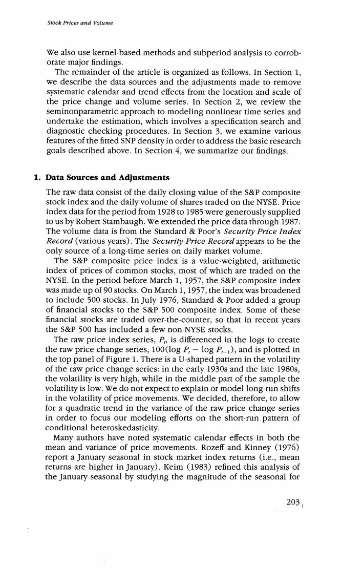
Stock Prices and Volume We also use kernel-based methods and subperiod analysis to corrob- orate major findings. The remainder of the article is organized as follows.In Section 1, we describe the data sources and the adjustments made to remove systematic calendar and trend effects from the location and scale of the price change and volume series.In Section 2,we review the seminonparametric approach to modeling nonlinear time series and undertake the estimation,which involves a specification search and diagnostic checking procedures.In Section 3,we examine various features of the fitted SNP density in order to address the basic research goals described above.In Section 4,we summarize our findings. 1.Data Sources and Adjustments The raw data consist of the daily closing value of the S&P composite stock index and the daily volume of shares traded on the NYSE.Price index data for the period from 1928 to 1985 were generously supplied to us by Robert Stambaugh.We extended the price data through 1987. The volume data is from the Standard Poor's Security Price Index Record(various years).The Security Price Record appears to be the only source of a long-time series on daily market volume. The S&P composite price index is a value-weighted,arithmetic index of prices of common stocks,most of which are traded on the NYSE.In the period before March 1,1957,the S&P composite index was made up of 90 stocks.On March 1,1957,the index was broadened to include 500 stocks.In July 1976,Standard Poor added a group of financial stocks to the s&P 500 composite index.Some of these financial stocks are traded over-the-counter,so that in recent years the S&P 500 has included a few non-NYSE stocks. The raw price index series,P,is differenced in the logs to create the raw price change series,100(log P:-log P,-1),and is plotted in the top panel of Figure 1.There is a U-shaped pattern in the volatility of the raw price change series:in the early 1930s and the late 1980s, the volatility is very high,while in the middle part of the sample the volatility is low.We do not expect to explain or model long-run shifts in the volatility of price movements.We decided,therefore,to allow for a quadratic trend in the variance of the raw price change series in order to focus our modeling efforts on the short-run pattern of conditional heteroskedasticity. Many authors have noted systematic calendar effects in both the mean and variance of price movements.Rozeff and Kinney (1976) report a January seasonal in stock market index returns (i.e.,mean returns are higher in January).Keim (1983)refined this analysis of the January seasonal by studying the magnitude of the seasonal for 203
The Review of Financial Studies /v 5 n 2 1992 Unadjusted Price Movements,100(log P-log P) 1930 1940 1950 1960 1970 1980 Adjusted Price Movements(Ap) 1930 1940 1950 1960 1970 1980 Figure 1 Time serles of unadjusted and adjusted price movements The top panel shows a time-series plot of the daily unadjusted price change series,100(log P,- log P).The data are daily from 1928 to 1987,16,127 observations.The bottom panel shows the adjusted price change series Ap,.The adjustments remove calendar effects and long-term trend on the basis of the regressions shown in Table 1.The adjusted series Ap,can reasonably be taken as stationary,which is required for use of the SNP estimator.See Section 1 for a discussion of the adjustments. various size-based portfolios of stocks.Keim finds that most of the seasonal is associated with the returns on small stocks in January. Constantinides (1984)points out that tax-related trading might occur around the turn of the year,but that some sort of irrationality on the part of investors would be required to induce systematic shifts in the mean of stock returns.Thus,we might expect to see a January-Decem- ber seasonal in the volume series even in the absence of a mean effect on prices.French (1980)notes a weekend effect in stock returns with lower-than-average returns on Monday.French and Roll (1986)study the variance of stock returns around weekends and exchange holi- days,and document shifts in the variance associated with these non- trading periods.Ariel (1988)has uncovered evidence of an intra- month pattern of higher returns in the first half of the month.Glosten, Jagannathan,and Runkle (1989)and Schwert (1990a)also find evi- 204

Stock Prices and Volume dence of monthly and daily seasonals in means and standard devia- tions of returns. In order to adjust for these documented shifts in both the mean and variance of the price and volume series,we perform a two-stage adjustment process in which systematic effects are first removed from the mean and then from the variance.We use the following set of dummy and time-trend variables in the adjustment regressions to capture these systematic effects: 1.Day-of-the-week dummies (one for each day,Tuesday through Saturday). 2.Dummy variables for each number of nontrading days preceding the current trading day (dummies for each of 1,2,3,and 4 nontrading days since the preceding trading day).These"gap"variables capture the effects of holidays and weekends.The distribution of these gaps in the trading record are as follows: gap of one nontrading day:1339 gap of two nontrading days:1873 gap of three nontrading days:223 gap of four nontrading days:5 3.Dummy variables for months of March,April,May,June,July, August,September,October,and November. 4.Dummy variables for each week of December and January.These variables are designed to accommodate the well-known "January' effect in both the mean and variance of prices and volume. 5.Dummy variables for each year,1941 to 1945. 6.t,t2,time trend variables.(Note:these variables are not included in the mean regressions for the price change.) This list of variables is generally self-explanatory,though we should elaborate on a few points concerning the "gap"variables in the sec- ond group.As to frequency,there are more one-day gaps and fewer two-day gaps than one might expect as a result of trading on Saturdays for the years 1928 through mid-year 1949.As to encoding,if trading occurred on the preceding day,then there is no gap in the trading record and no dummy is included;there are 12,686 such days.The Bank Holiday of 1933 is associated with a gap of 11 days over which the increase in the raw S&P index is the largest close-to-close move- ment in the entire data set.No dummy is included for this single 11- day gap because doing so would,in effect,replace the largest upward change in the price index with the unconditional mean of the price changes,which in our view would not accurately reflect what tran- spired over the Bank Holiday.Finally,in both the adjustments for the mean and variance of volume,the coefficients of the four gap variables 205
Tbe Review of Financial Studies /v 5 n 2 1992 are constrained to lie along a line.Without such constraints,the adjustment process itself appears to create some very extreme and implausible values in the adjusted volume process,particularly for the five days in which gap =4. To perform the adjustment,we first regress 100(log P:-log P1) or log(V)(V,represents volume)on the set of adjustment variables: w=xB+u (mean equation). Here w is the series to be adjusted and x contains the adjustment regressors.The least squares residuals are taken from the mean equa- tion to construct a variance equation: log(42)=x'y +e (variance equation). This regression is used to standardize the residuals from the mean equation,and then a final linear transformation is performed to cal- culate adjusted w: wadi a+b(i/exp(x'y/2)), where a and b are chosen so that the sample means and variances of w and wadi are the same.The linear transformation makes the units of measurement of adjusted and unadjusted data the same,which facilitates interpretation of our empirical results.In what follows,Ap. denotes adjusted 100(log P,-log P-1)and v,denotes adjusted log V.. Table 1 shows the estimated coefficients in the mean and variance adjustment equations for the price change series.The patterns confirm the well-known day-of-the-week and January effects:Monday has a lower return than any other day of the week,which is seen by noting that the coefficients of all other day-of-the-week dummies are positive. Price changes are higher in the last week of December and the first week of January.The effect of wartime seems to be confined to a reduction in the variance. The Ap,series is plotted in the bottom panel of Figure 1.The adjustments make the series appear more homogeneous,thereby allowing us to focus on the day-to-day dynamic structure under an assumption of stationarity. We do not regard the Ap,series as a market-returns series since the S&P index is not adjusted for dividend payout.If dividend payout is lumpy and the payout has an appreciable effect on the index (because of groups of stocks going ex-dividend together),then the lumpy dividends can create yet another possible systematic calendar effect. In order to investigate the lumpiness of dividend payout,we obtained daily data on the total dividend payout of the s&P 100 index in the period 1979 to 1987.[These data are used in Harvey and Whaley (1991),and we thank the authors for allowing us access to these data.] 206
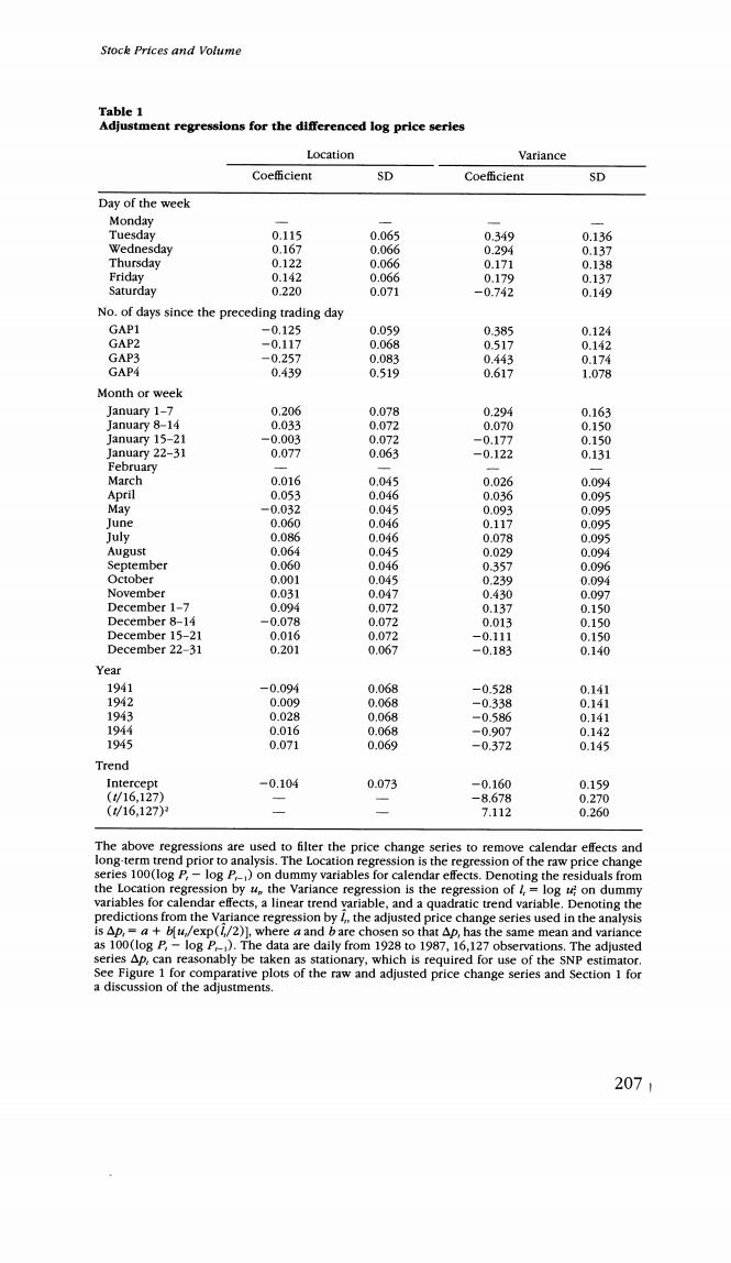
Stock Prices and Volume Table 1 Adjustment regressions for the differenced log price serles Location Variance Coefficient SD Coe伍cient SD Day of the week Monday Tuesday 0.115 0.065 0.349 0.136 Wednesday 0.167 0.066 0.294 0.137 Thursday 0.122 0.066 0.171 0.138 Friday 0.142 0.066 0.179 0.137 Saturday 0.220 0.071 -0.742 0.149 No.of days since the preceding trading day GAP1 -0.125 0.059 0.385 0.124 GAP2 -0.117 0.068 0.517 0.142 GAP3 -0.257 0.083 0.443 0.174 GAP4 0.439 0.519 0.617 1.078 Month or week January 1-7 0.206 0.078 0.294 0.163 January 8-14 0.033 0.072 0.070 0.150 January 15-21 -0.003 0.072 -0.177 0.150 January 22-31 0.077 0.063 -0.122 0.131 February March 0.016 0.045 0.026 0.094 April 0.053 0.046 0.036 0.095 May -0.032 0.045 0.093 0.095 lune 0.060 0.046 0.117 0.095 July 0.086 0.046 0.078 0095 August 0.064 0.045 0.029 0.094 September 0.060 0.046 0.357 0.096 October 0.001 0.045 0.239 0.094 November 0.031 0.047 0.430 0.097 December 1-7 0.094 0.072 0.137 0.150 December 8-14 -0.078 0.072 0.013 0.150 December 15-21 0.016 0.072 -0.111 0.150 December 22-31 0.201 0.067 -0.183 0.140 Year 1941 -0.094 0.068 -0.528 0.141 1942 0.009 0.068 -0.338 0.141 1943 0.028 0.068 -0.586 0.141 1944 0.016 0.068 =0.907 0.142 1945 0.071 0.069 -0.372 0.145 Trend Intercept -0.104 0.073 -0.160 0.159 (/16,127) -8.678 0.270 (16.127) 7.112 0.260 The above regressions are used to filter the price change series to remove calendar effects and long-term trend prior to analysis.The Location regression is the regression of the raw price change series 100(log P,-log P-)on dummy variables for calendar effects.Denoting the residuals from the Location regression by ue the variance regression is the regression of /,log u;on dummy variables for calendar effects,a linear trend variable,and a quadratic trend variable.Denoting the predictions from the Variance regression by the adjusted price change series used in the analysis is Ap,=a+bfu/exp(/2)],where a and b are chosen so that Ap,has the same mean and variance as 100(log P,-log P).The data are daily from 1928 to 1987,16,127 observations.The adjusted series Ap,can reasonably be taken as stationary,which is required for use of the SNP estimator See Figure 1 for comparative plots of the raw and adjusted price change series and Section 1 for a discussion of the adjustments. 207