Traditional models:path loss (1/4) Case 1)free-space Friis equation 2 Px=Pr GrGR Ro 4πR =Px(Ro) R Ro reference distance Therefore power Path Loss L increases with the square of link distance R 4πR =L(R) R Path Gain (PG)is the inverse of L PG=1/L=PR/P 8
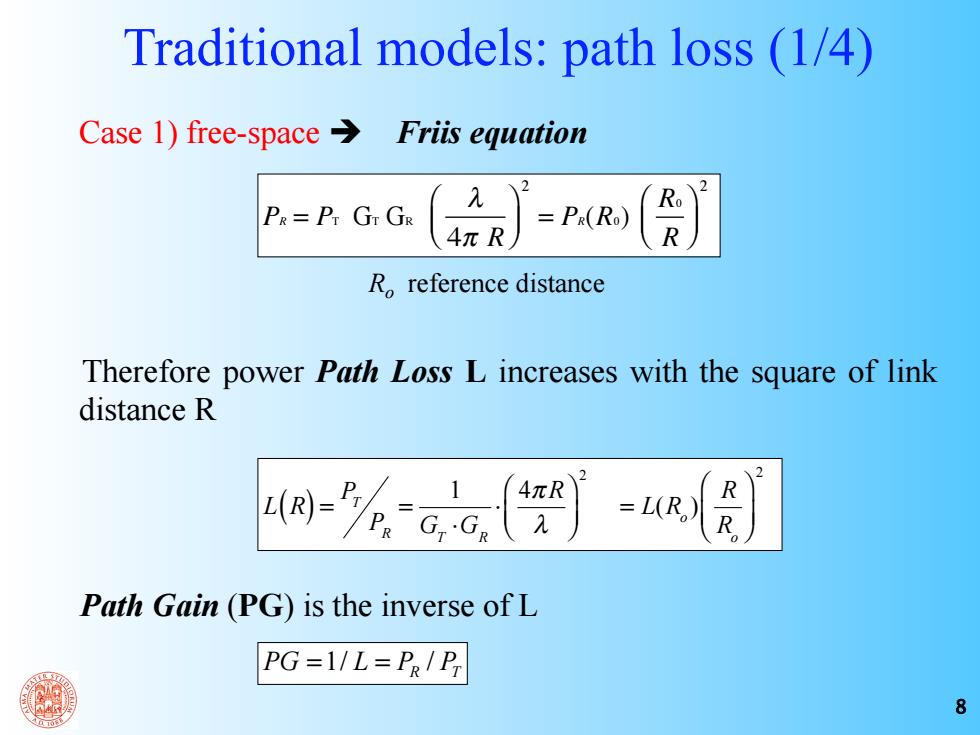
8 Traditional models: path loss (1/4) Case 1) free-space Friis equation Therefore power Path Loss L increases with the square of link distance R L(R) = PT PR = 1 GT ⋅GR ⋅ 4πR λ ⎛ ⎝ ⎜ ⎞ ⎠ ⎟ 2 = L(R o ) R R o ⎛ ⎝ ⎜ ⎞ ⎠ ⎟ 2 Path Gain (PG) is the inverse of L 1/ / PG = L = PR PT PR = PT GT GR λ 4π R ⎛ ⎝ ⎜ ⎞ ⎠ ⎟ 2 = PR(R0) R0 R ⎛ ⎝ ⎜ ⎞ ⎠ ⎟ 2 Ro reference distance
Traditional models:path loss (2/4) Expressing L in dB: L4R (R)=L4R (R)-10.2 logR+10.2 logR=K(f)+10.2 logR LdB in free space is logarithmic with R or LdB in free space is linear with log R.The line slope is determined by the exponent"2” LdB LdB “log-log graph'” log R
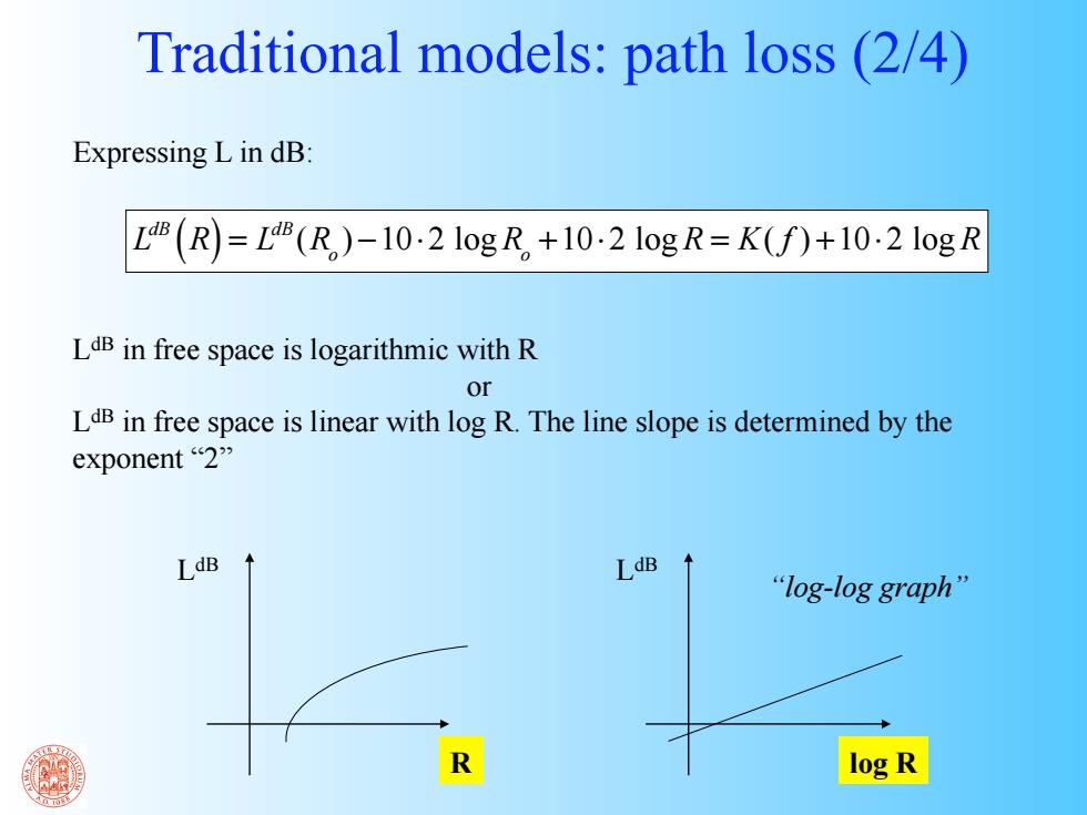
Expressing L in dB: LdB (R) = LdB (R o ) −10⋅2 log R o +10⋅2 log R = K( f ) +10⋅2 log R LdB in free space is logarithmic with R or LdB in free space is linear with log R. The line slope is determined by the exponent “2” LdB R LdB log R Traditional models: path loss (2/4) “log-log graph
Traditional models:path loss(3/4) Case 2)real environment> Hata-like models 40 L(1000) (R)=L(R,) R R。 2 100 Z(R)=K(f,)+10·a logR An attenuation law similar to free space is assumed but with a different exponent: a path loss exponent or path loss factor 0u>2 a is derived through fitting(regression line)on a set of measured path loss data →empirical modeling 10
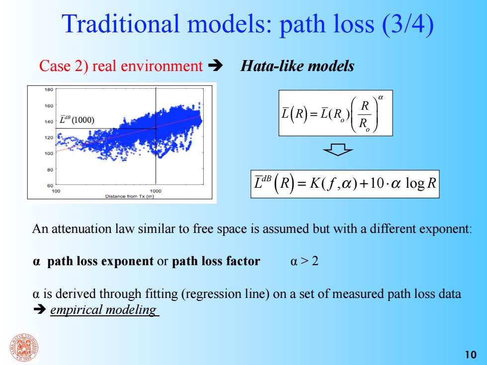
10 An attenuation law similar to free space is assumed but with a different exponent: α path loss exponent or path loss factor α > 2 α is derived through fitting (regression line) on a set of measured path loss data empirical modeling Traditional models: path loss (3/4) Case 2) real environment Hata-like models LdB (R) = K( f ,α) +10⋅α log R L(R) = L(R o ) R R o ⎛ ⎝ ⎜ ⎞ ⎠ ⎟ α
Traditional models:path loss (4/4) Hata-like models give the mean path loss Deviations from the mean value are called fading:slow fading (or shadowing) and fast fading (Rayleigh fading)and are usually described through statistical distributions statistical modeling (add)(T Bane nuno 'qold (ado)(Da F(L)=Prob L<L' 0.5 LdB LdB Average attenuation M Hata-like models→ empirical-statistical models 11
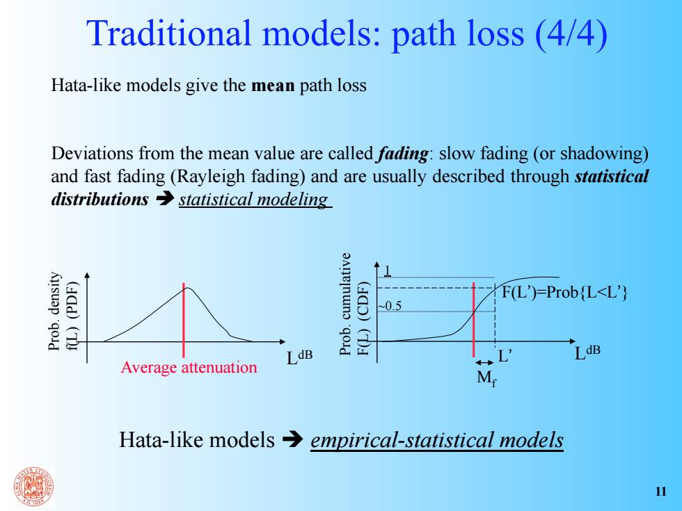
Hata-like models give the mean path loss Deviations from the mean value are called fading: slow fading (or shadowing) and fast fading (Rayleigh fading) and are usually described through statistical distributions statistical modeling Average attenuation Prob. density f(L) (PDF) Prob. cumulative F(L) (CDF) LdB ~0.5 1 LdB F(L’)=Prob{L<L’} L’ Traditional models: path loss (4/4) Mf Hata-like models empirical-statistical models 11
Other functional dependences of L However,in some cases not only achanges w.r.t.free space,but the overall functional dependance with R changes.Ex:indoors: Tx Rx office rooms L (R)=I4H (R)+IN=K+20logR- Multi-wall R model Ex:propagation through a lossy medium Specific attenuation [dB/m] L(R=L(R+[dBIm·R Linear model 12
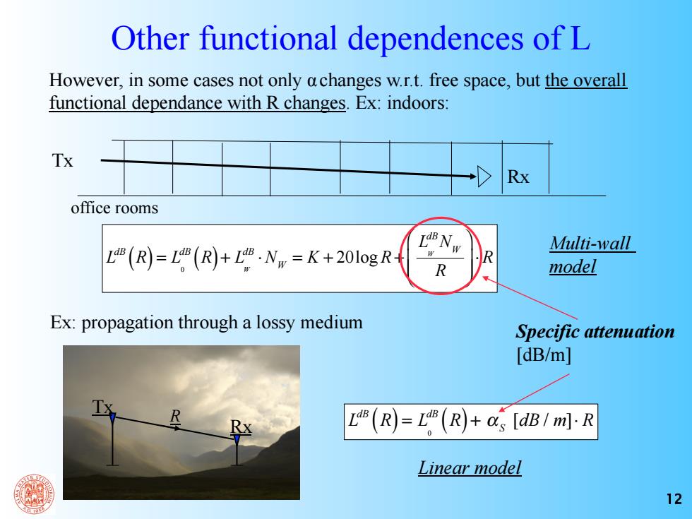
12 However, in some cases not only αchanges w.r.t. free space, but the overall functional dependance with R changes. Ex: indoors: Tx Rx office rooms LdB (R) = L 0 dB (R) + L W dB ⋅ NW = K + 20log R + L W dBNW R ⎛ ⎝ ⎜ ⎜ ⎞ ⎠ ⎟ ⎟ ⋅ R Specific attenuation [dB/m] Other functional dependences of L Ex: propagation through a lossy medium LdB (R) = L 0 dB (R) + α S R [dB / m]⋅ R Tx Rx Multi-wall model Linear model