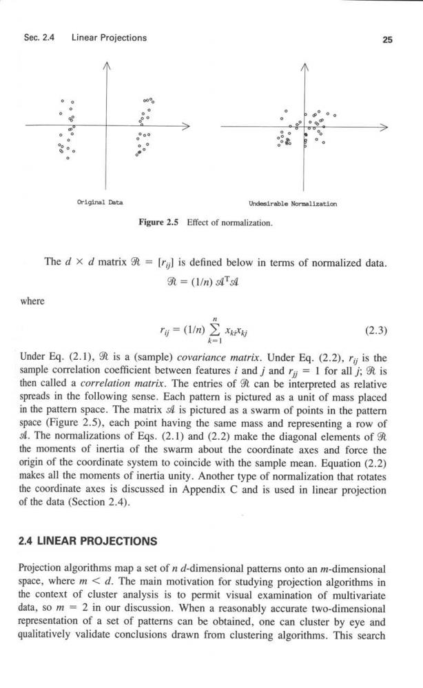
Sec.2.4 Linear Projections 25 Original Data Undesirable Normallzatlon Figure 2.5 Effect of normalization. The d x d matrix=[rgl is defined below in terms of normalized data. =(l/n)s4s4 where rg=(1/m) Xk对 (2.3) Under Eq.(2.1),g is a (sample)covariance matrix.Under Eq.(2.2),rij is the sample correlation coefficient between features i and j and ry=1 for all j;is then called a correlation matrix.The entries of 9 can be interpreted as relative spreads in the following sense.Each pattern is pictured as a unit of mass placed in the pattern space.The matrix is pictured as a swarm of points in the pattern space(Figure 2.5),each point having the same mass and representing a row of 4.The normalizations of Eqs.(2.1)and (2.2)make the diagonal elements of the moments of inertia of the swarm about the coordinate axes and force the origin of the coordinate system to coincide with the sample mean.Equation(2.2) makes all the moments of inertia unity.Another type of normalization that rotates the coordinate axes is discussed in Appendix C and is used in linear projection of the data(Section 2.4). 2.4 LINEAR PROJECTIONS Projection algorithms map a set of n d-dimensional patterns onto an m-dimensional space,where m<d.The main motivation for studying projection algorithms in the context of cluster analysis is to permit visual examination of multivariate data,so m =2 in our discussion.When a reasonably accurate two-dimensional representation of a set of patterns can be obtained,one can cluster by eye and qualitatively validate conclusions drawn from clustering algorithms.This search
26 Data Representation Chap.2 for a two-dimensional projection is closely related to problems in multivariate analysis of variance and factor analysis(see Appendices E and F). A linear projection expresses the m new features as linear combinations of the original d features. y:=就x fori=1,...,n Here,yi is an m-place column vector,x;is a d-place column vector,and is an m x d matrix.Linear projection algorithms are relatively simple to use,tend to preserve the character of the data,and have well-understood mathematical properties. The type of linear projection used in practice is influenced by the availability of category information about the patterns in the form of labels on the patterns.If no category information is available,the eigenvector projection (also called the Karhunen-Loeve method,or principal component method)is commonly used. Discriminant analysis is a popular linear mapping technique when category labels are available.We now describe these two popular linear projection algorithms. Readers will find some useful background information on linear algebra and scatter matrices in Appendices C and D. 2.4.1 Eigenvector Projection The eigenvectors of the covariance matrix 9 in Eq.(2.3)define a linear projection that replaces the features in the raw data with uncorrelated features. These eigenvectors also provide a link between cluster analysis and factor analysis (Appendix E).Since 9 is a d x d positive definite matrix,its eigenvalues are real and can be labeled so that 入1≥入2≥…≥入g≥0 A set of corresponding eigenvectors,c,c2....,c.is labeled accordingly. The m x d matrix of transformation is defined from the eigenvectors of the covariance matrix (or correlation matrix)9 as follows.The eigenvectors are also called principal components. 米m1 c The rows of are eigenvectors,as are the rows of Gg defined in Appendix C.This matrix projects the pattern space into an m-dimensional subspace (hence the subscript m on a)whose axes are in the directions of the largest eigenvalues of 9 as follows.The derivation is given in Section 2.4.2. y:=9光mX fori=1,...,n (2.4) The projected patterns can be written as follows:
Sec.2.4 Linear Projections 27 男m Note that x,is the original pattern and y;is the corresponding projected pattern. Equation (2.4)will be called the eigenvector transformation. The covariance matrix in the new space can be defined with Eq.(C.1)as follows: (1/m)3男nm=(1/m)∑yyT=3光T=9 e6RAR(3孔ne3) i=1 The matrix can be partitioned as follows,where is an m x m identity matrix and O is an m x (d-m)zero matrix. 光mR=[o Thus the covariance matrix in the new space,Am,becomes a diagonal matrix as shown below. (1/m)83m=Λm=diag(1,入2,···,入m) (2.5) This implies that the m new features obtained by applying the linear transformation defined by are uncorrelated. Techniques for choosing an appropriate value for m in Eq.(2.4)are based on the eigenvalues of 9.Comparing Eqs.(C.2)and(2.5)shows that the sum of the first m eigenvalues is the "'variance''retained in the new space.That is,the eigenvalues of g are the sample variances in the new space,while the sum of the d eigenvalues is the total variance in the original pattern space.Since the eigenvalues are ordered largest first,one could choose m so that m=2/x≥0.95 which would assure that 95%of the variance is retained in the new space.Thus a"good''eigenvector projection is that which retains a large proportion of the variance present in the original feature space with only a few features in the transformed space.Krzanowski (1979)provides a table for the distribution of this ratio for m 1.d =3 and 4,and several values of n under the assumption that all components of all patterns are samples from independent standard normal distributions.These tables should help determine whether it is reasonable to say that the size of the largest eigenvalue could have been achieved by chance.Another technique for choosing m is to plot rm as a function of m and look for a"knee' in the plot
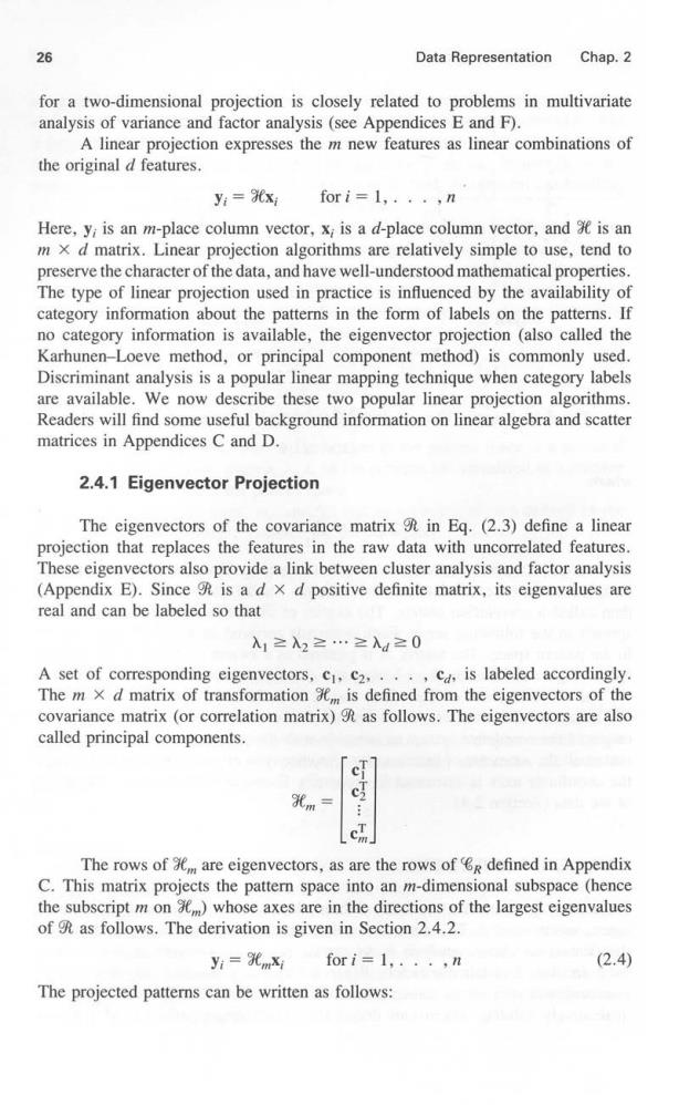
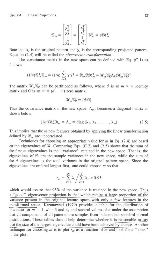
28 Data Representation Chap.2 Example 2.5 This example shows the eigenvector projection on the 80X data set described in Example 2.1.The pattern matrix is normalized by subtracting the sample means [Eg.(2.1)].The normalized data are projected to two dimensions(m =2)with Eq.(2.4)as shown in Figure 2.6,where category labels are given for the projected patterns.The percentage variance retained in two dimensions is 43.1%.A factor analysis (Appendix E)shows that features 5 to 8 most strongly affect the first coordinate (abscissa in Figure 2.6).Since these features are horizontal and vertical measurements (Figure 2.1),we could name the abscissa in Figure 2.6 as "horizontal-vertical.'Features 2,3.6,7,and 8 most strongly affect the second projected feature (ordinate in Figure 2.6).so we could name the axis "rightside. Subsequent clusterings of the 8OX data will show that the patterns are separated quite well according to category.Some of this separation is evident in Figure 2.6.To demonstrate how the first two principal components of the 80X data exhibit more structure than other principal components,we show the projection defined by the third and fourth principal components,or the eigenvectors correspond- ing to the third and fourth largest eigenvalues of,in Figure 2.7.Little separation 00 00 8 88 00 00 800 88 0 00 80 8 88 8 X X X X Figure 2.6 Two-dimensional representation of 80X data on the first two principal components
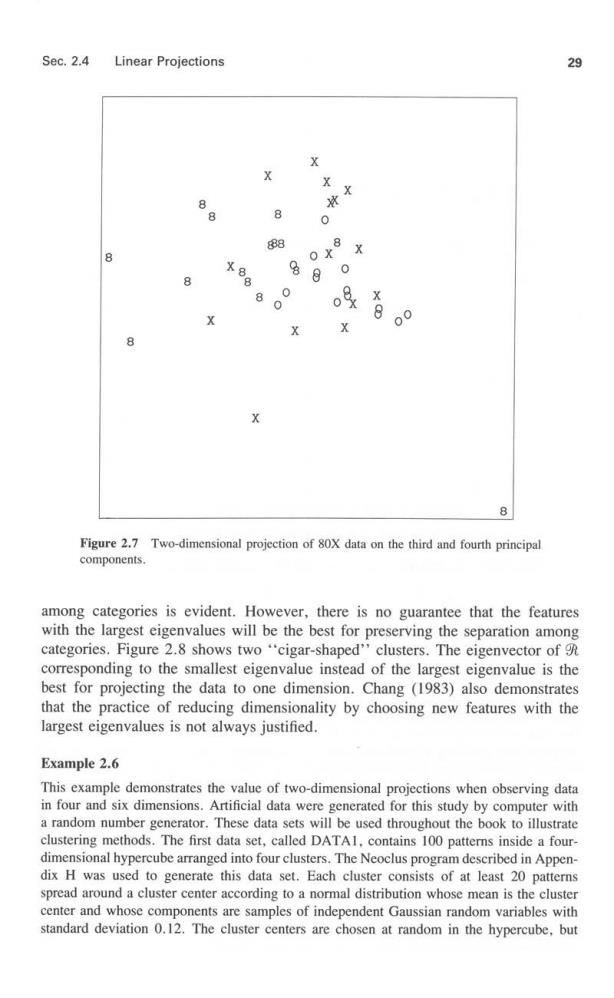
Sec.2.4 Linear Projections 29 X X X 8 0 88 e 486 O x %8 0 8 8 0 8 0 中 8 X 00 X K 8 Figure 2.7 Two-dimensional projection of 80X data on the third and fourth principal components. among categories is evident.However,there is no guarantee that the features with the largest eigenvalues will be the best for preserving the separation among categories.Figure 2.8 shows two "cigar-shaped''clusters.The eigenvector of corresponding to the smallest eigenvalue instead of the largest eigenvalue is the best for projecting the data to one dimension.Chang (1983)also demonstrates that the practice of reducing dimensionality by choosing new features with the largest eigenvalues is not always justified. Example 2.6 This example demonstrates the value of two-dimensional projections when observing data in four and six dimensions.Artificial data were generated for this study by computer with a random number generator.These data sets will be used throughout the book to illustrate clustering methods.The first data set,called DATAI.contains 100 patterns inside a four- dimensional hypercube arranged into four clusters.The Neoclus program described in Appen- dix H was used to generate this data set.Each cluster consists of at least 20 patterns spread around a cluster center according to a normal distribution whose mean is the cluster center and whose components are samples of independent Gaussian random variables with standard deviation 0.12.The cluster centers are chosen at random in the hypercube,but