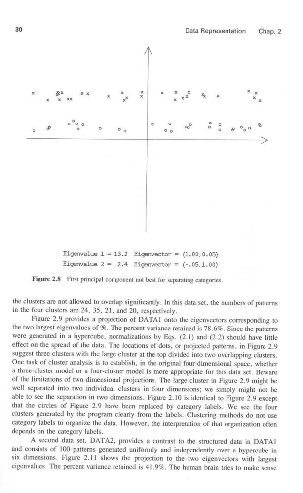
30 Data Representation Chap.2 XX oo 88 Eigenvalue 1 13.2 Eigenvector (1.00,0.05) Eigenvalue 2 2.4 Eigenvector =(-.05,1.00) Figure 2.8 First principal component not best for separating categories. the clusters are not allowed to overlap significantly.In this data set,the numbers of patterns in the four clusters are 24,35,21,and 20,respectively. Figure 2.9 provides a projection of DATAI onto the eigenvectors corresponding to the two largest eigenvalues of g.The percent variance retained is 78.6%.Since the patterns were generated in a hypercube,normalizations by Egs.(2.1)and(2.2)should have little effect on the spread of the data.The locations of dots,or projected patterns,in Figure 2.9 suggest three clusters with the large cluster at the top divided into two overlapping clusters. One task of cluster analysis is to establish,in the original four-dimensional space,whether a three-cluster model or a four-cluster model is more appropriate for this data set.Beware of the limitations of two-dimensional projections.The large cluster in Figure 2.9 might be well separated into two individual clusters in four dimensions;we simply might not be able to see the separation in two dimensions.Figure 2.10 is identical to Figure 2.9 except that the circles of Figure 2.9 have been replaced by category labels.We see the four clusters generated by the program clearly from the labels.Clustering methods do not use category labels to organize the data.However,the interpretation of that organization often depends on the category labels. A second data set,DATA2,provides a contrast to the structured data in DATAl and consists of 100 patterns generated uniformly and independently over a hypercube in six dimensions.Figure 2.1I shows the projection to the two eigenvectors with largest eigenvalues.The percent variance retained is 41.9%.The human brain tries to make sense
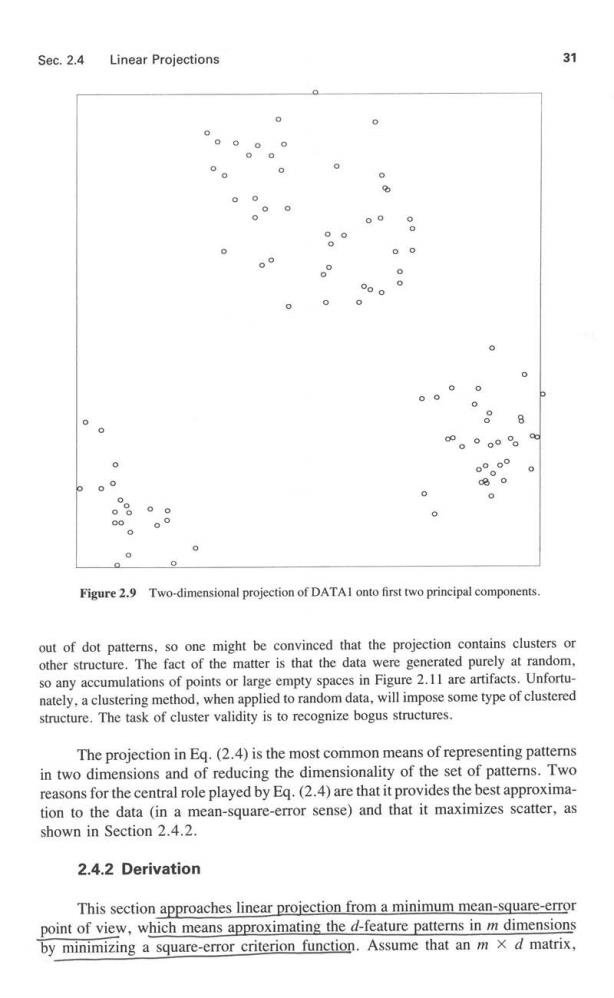
Sec.2.4 Linear Projections 31 0 000 0 0 0 0 8 8 。°og 6 00 8 0 0 00 00 0 Figure 2.9 Two-dimensional projection of DATAI onto first two principal components. out of dot patterns,so one might be convinced that the projection contains clusters or other structure.The fact of the matter is that the data were generated purely at random, so any accumulations of points or large empty spaces in Figure 2.11 are artifacts.Unfortu- nately,a clustering method,when applied to random data,will impose some type of clustered structure.The task of cluster validity is to recognize bogus structures. The projection in Eg.(2.4)is the most common means of representing patterns in two dimensions and of reducing the dimensionality of the set of patterns.Two reasons for the central role played by Eq.(2.4)are that it provides the best approxima- tion to the data (in a mean-square-error sense)and that it maximizes scatter,as shown in Section 2.4.2. 2.4.2 Derivation This section approaches linear projection from a minimum mean-square-error point of view,which means approximating the d-feature patterns in m dimensions by minimizing a square-error criterion function.Assume that an m x d matrix
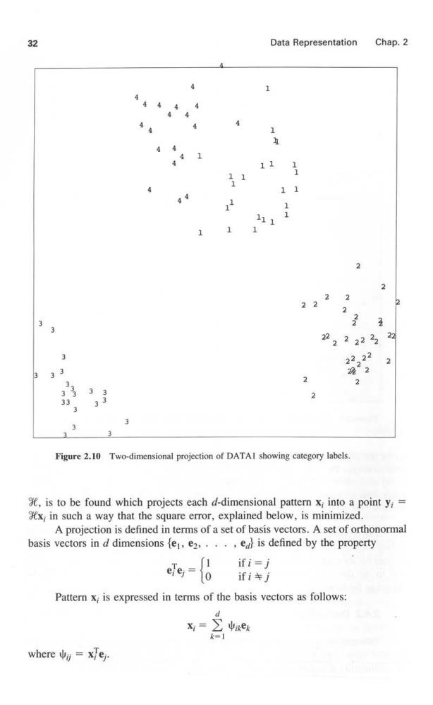
32 Data Representation Chap.2 4 1 11 1 11 1 111 1 2 2 2222 子 3 22 22222 22 2222 3 3 3 22”2 2 2 33 Figure 2.10 Two-dimensional projection of DATAI showing category labels. is to be found which projects each d-dimensional pattern x;into a point y; x;in such a way that the square error,explained below,is minimized. A projection is defined in terms of a set of basis vectors.A set of orthonormal basis vectors in d dimensions fe,e2,...,edl is defined by the property g= ifi=j ifij Pattern x;is expressed in terms of the basis vectors as follows: d e where=xfej
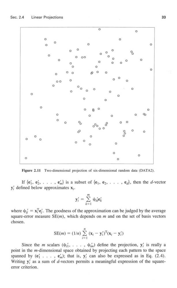
Sec.2.4 Linear Projections 33 0 0 0 8 00 0 0 0 0 0 0 0 0 。0 0 0 0 0 0 0 0 0 0 % 00 8 0 0 0 0 Figure 2.11 Two-dimensional projection of six-dimensional random data (DATA2). If{ei,ei,··,em}is a subset of{e,e2,···,el,then the d-vector y defined below approximates x;. k=1 where=xe.The goodness of the approximation can be judged by the average square-error measure SE(m),which depends on m and on the set of basis vectors chosen. SE(m)=(I/n)(x;-yi)(x:-y) = Since the m scalars(他i,··,,im)define the projection,yi is really a point in the m-dimensional space obtained by projecting each pattern to the space spanned by (ef...,em);that is,y can also be expressed as in Eq.(2.4). Writing y as a sum of d-vectors permits a meaningful expression of the square- error criterion
34 Data Representation Chap.2 A set of basis vectors that minimizes SE(m)has been shown to be a set of eigenvectors (c,...,c)for the covariance matrix (Tou and Heydorn, 1967;Sebestyen,1962;Wilks,1963;Fukunaga.1972).In addition,the basis vectors that minimize SE(m)correspond to the m largest eigenvalues of.Projecting x;into this optimal subspace is precisely the operation in Eq.(2.4).The degree of approximation can be determined by expressing the minimum square error in terms of eigenvalues of SE(m)min This result justifies the rule suggested earlier for choosing m.Retaining only those new features that provide the largest spreads minimizes the square error.In other words,the importance,in a square-error sense,of each prospective new feature is measured by an eigenvalue of 9.The normalization of Eq.(2.2) scales the pattern space so that A;=d,but the development given above is wholly applicable. The second reason for the importance of Eg.(2.4)is that the eigenvector projection maximizes scatter.This interpretation of Eq.(2.4)has its roots in theoreti- cal statistics (Wilks,1963).Assuming normalization by Eq.(2.1)or (2.2),the scatter of the set of patterns is given by 9=n别 where is the determinant of the covariance matrix,9. Wilks (1963)has provided a geometrical interpretation of scatter.Another interpretation follows from the relation between S and 9.From Eg.(C.2), i=1 This shows that the scatter is invariant through a rotation of the pattern space, such as Eq.(2.4)when m =d.A set of eigenvalues for 9 is also a set for More important,it shows that the scatter is proportional to the product of the sample variances(,···,入d)along the rotated axes. If the patterns are projected into an m-dimensional space by Eq.(2.4),their scatter is maximized in the m-dimensional space with respect to all other orthogonal m-dimensional projections because Eq.(2.4)uses eigenvectors corresponding to the m largest eigenvalues of(or of )From an intuitive point of view,maximizing scatter might not appear to be as worthy a goal as minimizing square error,although both are achieved with the same transformation. 2.4.3 Discriminant Analysis Classical discriminant analysis (Wilks,1963:Friedman and Rubin,1967; Fortier and Solomon,1966;Lachenbruch and Goldstein,1979)attempts to project patterns into a space having fewer dimensions than the original pattern space