20 Data Representation Chap.2 Then the distance between x;and xe is written as d(i,k)= 之9 where do is the number of features missing in x;or xy or both.Note that if there are no missing values,then d(i,k)defined above is the squared Euclidean distance. 4.Let d,denote the average distance between all pairs of patterns along the jth feature defined as follows: d=n n-1)2 where n is the number of patterns.Now define the distance between two patterns along the ith feature as 4= d, ifxy or xy is missing otherwise Finally,the distance between patterns x,and xe is written as di,=∑明 Based on experimental results,Dixon (1979)recommends method 3 as the best overall method. 2.2.4 Probabilistic Indices Goodall(1966)proposed an index of similarity that has a uniform distribution when the data are "random.''The idea of using a probability scale to assess the significance of a proximity measure appears in Hamdan and Tsokos(1971),who define an information measure for a contingency table,and Brockett et al.(1981), who used the asymptotic distribution of an information-theoretic measure on ques- tionnaire data.Li (1984)provided the most recent example of this type of measure. Before explaining the proximity measure,we reexamine the simple matching and Jaccard coefficients in light of their distributions under "random''data. Matching coefficients measure the degree of similarity between objects.We know that their value is between 0 and I but do not know how large a value is required before two objects can be called "'close.''We now examine baseline distributions for the simple matching coefficient and the Jaccard coefficient.A baseline distribution describes a state of"randomness,''or the absence of structure, for gauging the magnitude of a matching coefficient.Baseline distributions are used extensively in Chapter 4.Two vectors will be called "'close''if a similarity as large as the one observed is unlikely under a baseline distribution. The simple matching coefficient between two d-position binary vectors a and b can be expressed as
Sec.2.2 Proximity Indices 27 SMC(a,b)=(1/d)(number of positions in which a and b match) A value z of SMC can be considered to be "'unusually''large if the probability of achieving a value of z or more is sufficiently low under some baseline distribution, such as the distribution of SMC for two randomly selected d-vectors.The choice of a baseline distribution is a matter of taste and depends on the application.The population o is defined as the set of all 4d possible pairs of d-vectors.The probability function Po assigns probability 4 to each pair in o and provides an obvious baseline distribution.This is equivalent to filling in the d-vectors by choosing the I's and 0's independently with probability 1/2,as in d flips of a true coin.It is easy to show that the distribution of SMC follows the binomial distribution(Appendix B).Thus the probability that SMC is k/d or more can be written as PoI[SMC(a,b)≥kd= )2 The notation d m denotes the binomial coefficient or d d m m!(d-m)! For example,the probability that two six-position,randomly chosen binary vectors match in four or more positions (i.e.,SMC 2/3)is 0.3438,while the chance that SMC is 5/6 or more is 0.1094.Thus a value as large as 2/3 for SMC when d 6 is not too unlikely even when there is no inherent correspondence between the vectors.A value of 5/6 might be required before calling the vectors unusually close under this baseline distribution.Even a perfect match has probability 0.0156, so one can never be absolutely sure that a large similarity is not a purely random event. The Jaccard coefficient for two d-position vectors is given below,where 0 is the vector containing all zeros. number of 1-1 matches J(a,b)= if(a,b)≠(0,0) d-Number of 0-0 matches J0,0)=1 The baseline distribution for J cannot be stated as compactly as that for SMC. Po≥)=∑∑Po1k,m where
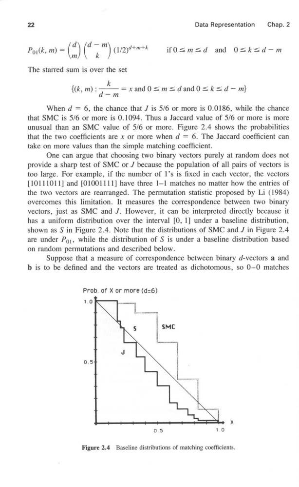
22 Data Representation Chap.2 Por(k,m) m 、k (1/2)4+m+ if0≤m≤dand0≤k≤d-m The starred sum is over the set k {k,m) =xand0≤m≤dand0≤k≤d-ml d-m When d=6,the chance thatJ is 5/6 or more is 0.0186,while the chance that SMC is 5/6 or more is 0.1094.Thus a Jaccard value of 5/6 or more is more unusual than an SMC value of 5/6 or more.Figure 2.4 shows the probabilities that the two coefficients are x or more when d =6.The Jaccard coefficient can take on more values than the simple matching coefficient. One can argue that choosing two binary vectors purely at random does not provide a sharp test of SMC or J because the population of all pairs of vectors is too large.For example,if the number of I's is fixed in each vector,the vectors [10111011]and [01001111]have three I-1 matches no matter how the entries of the two vectors are rearranged.The permutation statistic proposed by Li (1984) overcomes this limitation.It measures the correspondence between two binary vectors,just as SMC and J.However,it can be interpreted directly because it has a uniform distribution over the interval [0,1]under a baseline distribution, shown as S in Figure 2.4.Note that the distributions of SMC and J in Figure 2.4 are under Po,while the distribution of S is under a baseline distribution based on random permutations and described below. Suppose that a measure of correspondence between binary d-vectors a and b is to be defined and the vectors are treated as dichotomous,so 0-0 matches Prob.of x or more(d=6) 1.0 0. 0.5 1,0 Figure 2.4 Baseline distributions of matching coefficients
Sec.2.3 Normalization 23 are not as important as 1-1 matches.Consider the population o2 of all d!pairs of vectors that can be obtained by permuting the entries of one of the vectors. Not all pairs of vectors are distinct.Probability function Po2 assigns each pair of vectors probability mass 1/d!,thus establishing a new baseline distribution. Let Au be the number of 1-1 matches in a randomly selected pair of vectors from population o2.Let N be the number of I's in a and let N,be the number of I's in b.All pairs of vectors in o2 have N and Np I's.For example,there are six I's in [10111011].The probability that A=k can be obtained from the hypergeometric distribution(Appendix B)under Po2.In the notation of Appendix B,we have a population of size d with N defectives and we take a sample of size N.Of course,the roles of N and N,can be reversed.The probability of exactly k matches between pairs of I's is P02(A11=k) =H(k,Na,Np,d) This probability expression requires that max{0,Na+Wb-d}≤k≤min (Na,Nb} The S-statistic defined below is essentially the inverse of the hypergeometric cumulative density function.Such statistics have been used elsewhere(Kempthorne, 1952).The additive factor ensures that S has a (continuous)uniform distribution over the unit interval since U is a continuous uniform random variable over the unit interval.If t is the number of 1-1 matches observed between d-vectors a and b,the S-measure of proximity is S(a,b)=>H(d,Na,No.k)+H(d,Na,No,t)U k< Since the distribution of S is uniform under Po2,the value of S is implicitly meaningful.For example,the probability that S is z or more is I -z for z between 0 and 1,as shown in Figure 2.4.This proximity has been used in the analysis of questionnaire data (Li and Dubes,1984)and in a template-matching problem (Li and Dubes,1985).The additive factor does not contribute much to the value of S except when d is small. 2.3 NORMALIZATION Suppose that the raw data consist of an n x d pattern matrix in which all features are continuous and on a ratio scale.Raw data,or the actual measurements,are seldom used just as they are recorded unless a probabilistic model for pattern generation is available.Some normalization is usually employed based on the requirements of the analysis.Preparing the data for a cluster analysis requires
24 Data Representation Chap.2 some sort of normalization that takes into account the measure of proximity.For example,Euclidean distance is a popular and familiar index of dissimilarity,but it implicitly assigns more weighting to features with large ranges than to those with small ranges.Scaling one feature in miles and a second feature in inches makes the second feature numerically overpower the first.We present a normaliza- tion scheme that remedies some of these problems. As explained earlier in this section,the basic unit of data is called a pattern, denoted by a d-vector,whose components are scalars called features.The ith pattern is denoted by the (column)vector x in this section and the jth feature value for the ith pattern is denoted byxThe asterisk denotes"raw'or unnormalized data.If n is the number of patterns in the analysis,the pattern matrix is the n x d matrix 4: xixi2… s4”=[xix2 … X21X22 22 Each row of is a pattern.Each point in the pattern space is a potential pattern.We treat the case when n>d,so the patterns are visualized as a number of points scattered around the pattern space. The jth feature average,mj,and jth feature variance,,are defined as the sample mean and the sample variance for the ith feature. =(m i=1 号=(m)Σ(好-m2 i=1 The simplest type of normalization subtracts the feature means: =有-m吲 (2.1) This normalization makes feature values invariant to rigid displacements of the coordinates.The second type of normalization translates and scales the axes so that all the features have zero mean and unit variance: =垃二四 (2.2) Removing the asterisk indicates that the pattern has been normalized,but the type of normalization must be clear from the context.Other types of normalization include scaling by the range (Carmichael et al.,1968)and a heterogeneity measure (Hall,1969).Lumelsky (1982)incorporates the normalization into the clustering procedure.Normalization or scaling is not always desirable.For example,if the spread among the patterns is due to the presence of clusters,the normalization in Eq.(2.2)can change the interpoint distances and can alter the separation between natural clusters as demonstrated in Figure 2.5