
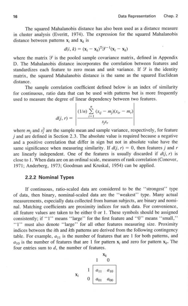
Sec.2.2 Proximity Indices 15 4.d(i,k)=0 only if xi=x 5.d(i,k)d(i,m)+d(m,k),all (i,k,m) Gower and Legendre(1986)show that for a metric dissimilarity matrix [d(i,)] only properties I and 4 are required;other properties can be derived from these two. The three most common Minkowski metrics are defined below and are illus- trated in Figure 2.3. ¥2 Euclidean Distance:[222/24.472 Manhattan Distance:4.2 =6 Sup Distance:Max (4,2)=4 ¥22 2 21 Figure 2.3 Minkowski metrics. 1.r =2(Euclidean distance) di, [-w=-- 2.r=1 (Manhattan,or taxicab,or city block distance) dik)=】 3.r→o'sup'distance) di,月=四整-xd Euclidean distance is the most common of the Minkowski metrics.The familiar geometric notions of invariance to translations and rotations of the pattern space are valid only for Euclidean distance.Accepted practice in the application area strongly affects the choice of proximity index.Euclidean distance seems to be preferred in engineering work.When all features are binary,the Manhattan metric is called the Hamming distance.or the number of features in which two patterns differ.Not all proximities encountered in applications are metrics.Tversky (1977)gives several examples to illustrate why a similarity is not always symmetric or transitive
16 Data Representation Chap.2 The squared Mahalanobis distance has also been used as a distance measure in cluster analysis (Everitt,1974).The expression for the squared Mahalanobis distance between patterns x;and x is di,)=(x-x)T9-'(x-x) where the matrix S is the pooled sample covariance matrix,defined in Appendix D.The Mahalanobis distance incorporates the correlation between features and standardizes each feature to zero mean and unit variance.If is the identity matrix,the squared Mahalanobis distance is the same as the squared Euclidean distance. The sample correlation coefficient defined below is an index of similarity for continuous,ratio data that can be used with patterns but is more frequently used to measure the degree of linear dependency between two features. (1/m)∑ (xii-mi)(xir -m,) d0i,r)= i=I where m;and sare the sample mean and sample variance,respectively,for feature jand are defined in Section 2.3.The absolute value is required because a negative and a positive correlation that differ in sign but not in absolute value have the same significance when measuring similarity.If d(j,r)=0,then features j and r are linearly independent.One of the features is usually discarded if d(j,r)is close to 1.When data are on an ordinal scale,measures of rank correlation(Conover, 1971;Anderberg,1973;Goodman and Kruskal,1954)can be applied. 2.2.2 Nominal Types If continuous,ratio-scaled data are considered to be the "strongest''type of data,then binary,nominal-scaled data are the "weakest'type.Many actual measurements,especially data collected from human subjects,are binary and nomi- nal.Matching coefficients are proximity indices for such data.For convenience, all feature values are taken to be either 0 or 1.These symbols should be assigned consistently;if“I'means“large'for the first feature and“O'means“small,'" 1''must also denote "'large''for all other features measuring size.Proximity indices between the ith and kth patterns are derived from the following contingency table.For example,a is the number of features that are I for both patterns,and ao is the number of features that are 1 for pattern x;and zero for pattern xy.The four entries sum to d,the number of features. Xk 1 0 a11 a10 dol a00
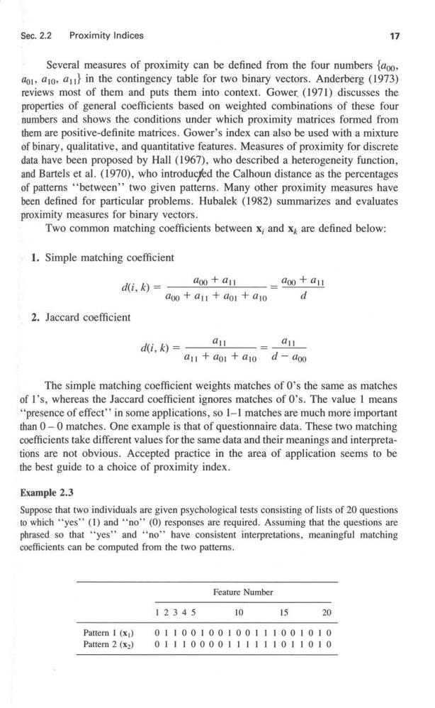
Sec.2.2 Proximity Indices 17 Several measures of proximity can be defined from the four numbers aoo. do,a1o,a in the contingency table for two binary vectors.Anderberg(1973) reviews most of them and puts them into context.Gower (1971)discusses the properties of general coefficients based on weighted combinations of these four numbers and shows the conditions under which proximity matrices formed from them are positive-definite matrices.Gower's index can also be used with a mixture of binary,qualitative,and quantitative features.Measures of proximity for discrete data have been proposed by Hall(1967),who described a heterogeneity function, and Bartels et al.(1970),who introducted the Calhoun distance as the percentages of patterns "between''two given patterns.Many other proximity measures have been defined for particular problems.Hubalek (1982)summarizes and evaluates proximity measures for binary vectors. Two common matching coefficients between x;and xy are defined below: 1.Simple matching coefficient d(i,k)= aoo +ai =doo+a1 ao0+a11+ao1+a10 d 2.Jaccard coefficient d(i,k)= a11 411 a1+ao aio d-doo The simple matching coefficient weights matches of 0's the same as matches of I's,whereas the Jaccard coefficient ignores matches of 0's.The value I means "presence of effect"'in some applications,so 1-1 matches are much more important than 0-0 matches.One example is that of questionnaire data.These two matching coefficients take different values for the same data and their meanings and interpreta- tions are not obvious.Accepted practice in the area of application seems to be the best guide to a choice of proximity index. Example 2.3 Suppose that two individuals are given psychological tests consisting of lists of 20 questions to which "yes''(1)and"'no''(0)responses are required.Assuming that the questions are phrased so that "yes''and "'no"have consistent interpretations,meaningful matching coefficients can be computed from the two patterns. Feature Number 12345 10 15 20 Pattern I (x) 01100100100111001010 Pattern 2(x2) 01110000111111011010

18 Data Representation Chap.2 The matching coefficients are derived from the following table: X2 0 Simple matching coefficients:15/20 0.75 Jaccard coefficient:8/13 =0.615 A value of I for either coefficient would mean identical patterns.However,other values are not as easily interpreted. Example 2.4 Suppose that two partitions of nine numerals are given and a measure of their proximity is desired. 61={1,3,4,5)(2,6),(7),(8,9)} 62={1,2,3,4),(5,6),7,8,9)} The characteristic function for a partition assigns the number I or 0 to a pair of numerals as follows. 7Ti,)= if numerals i and j are in the same subset in the partition 10 if not The characteristic functions T,andT2,for partitions€,and€2,respectively,are listed below in matrix form;T is shown above the diagonal and 72 is shown below the diagonal. 123456789 1-0111000 0 2 1 000 1 00 0 3 0 0 0 0 0 0 5 0 0 0 0 0 6 0 0 0 0 7 0 0 0 00 0 0 0 00 000 01-1 9 00 000011 The two characteristic functions are matched term by term to obtain the following table and coefficients.The relative significance of these values is discussed in the next section

Sec.2.2 Proximity Indices 19 T 10 6 0 22 Simple matching coefficient:26/36 0.722 Jaccard coefficient:4/14 0.286 2.2.3 Missing Data The problem of missing observations occurs often in practical applications. Suppose that some of the pattern vectors have missing feature values,as in xi=(xn x2?X4?6)T where the third and fifth features have not been recorded for the ith pattern. Missing values occur because of recording error,equipment failure,the reluctance of subjects to provide information,carelessness,and unavailability of information. Should incomplete pattern vectors be discarded?Should missing values be replaced by averages or nominal values?Answers to these questions depend on the size of the data set and the type of analysis.Sneath and Sokal (1973),Kittler (1978). Dixon(1979),and Zagoruiko and Yolkina(1982)all treat the problem of missing data. Dixon(1979)describes several simple,inexpensive,easy to implement,and general techniques for handling missing values.These techniques either eliminate part of the data,estimate the missing values,or compute an estimated distance between two vectors with missing values.We summarize some of these techniques here. 1.Simply delete the pattern vectors or features that contain missing values. This technique does not lead to the most efficient utilization of the data and should be used only in situations where the number of missing values is very small. 2.Suppose that the jth feature value in the ith pattern vector is missing.Find the K nearest neighbors of x;and replace the missing value xi by the average of the jth feature of the K nearest neighbors.The value of K should be a function of the size of the pattern matrix. 3.The distance between two vectors x;and xy containing missing values is computed as follows.First define the distance d,between the two patterns along the ith feature. 0 4= if xy or xy is missing x时一x为 otherwise