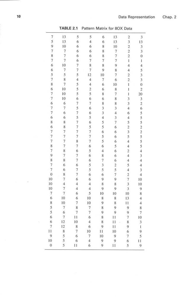
10 Data Representation Chap.2 TABLE 2.1 Pattern Matrix for 80X Data 13 13 2 5666667754 6688878907 10 7779876 759787665786776776867778798770000768556671900 30777075870006766887777878668747700767228555 546667872442567665657776566556644500 6 55567575777787677677644667 87 7 6868334556556487356989089898891099 08788343766665666257989088991110991 32221442211133464523544244542733031997896765 333301453302032655522555434434009844870319519 1087661 6460746
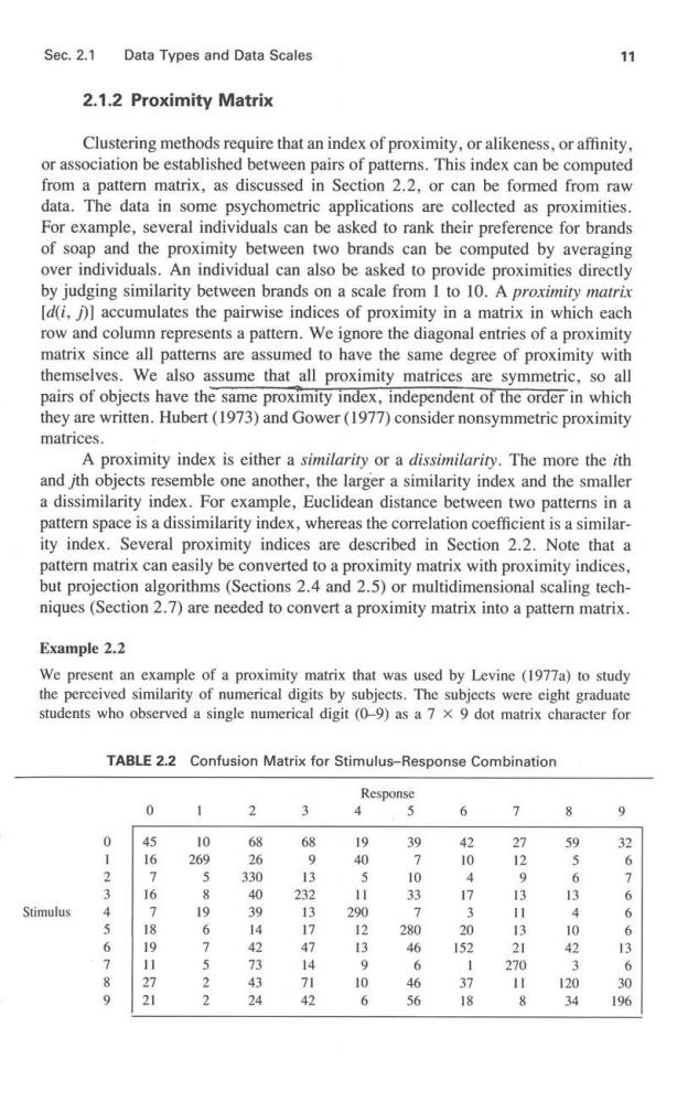
Sec.2.1 Data Types and Data Scales 11 2.1.2 Proximity Matrix Clustering methods require that an index of proximity,or alikeness,or affinity. or association be established between pairs of patterns.This index can be computed from a pattern matrix,as discussed in Section 2.2,or can be formed from raw data.The data in some psychometric applications are collected as proximities For example,several individuals can be asked to rank their preference for brands of soap and the proximity between two brands can be computed by averaging over individuals.An individual can also be asked to provide proximities directly by judging similarity between brands on a scale from I to 10.A proximiry matrix [d(i,accumulates the pairwise indices of proximity in a matrix in which each row and column represents a pattern.We ignore the diagonal entries of a proximity matrix since all patterns are assumed to have the same degree of proximity with themselves.We also assume that all proximity matrices are symmetric,so all pairs of objects have the same proximity index,independent of the order in which they are written.Hubert(1973)and Gower(1977)consider nonsymmetric proximity matrices. A proximity index is either a similariry or a dissimilariry.The more the ith and jth objects resemble one another,the larger a similarity index and the smaller a dissimilarity index.For example,Euclidean distance between two patterns in a pattern space is a dissimilarity index,whereas the correlation coefficient is a similar- ity index.Several proximity indices are described in Section 2.2.Note that a pattern matrix can easily be converted to a proximity matrix with proximity indices, but projection algorithms(Sections 2.4 and 2.5)or multidimensional scaling tech- niques(Section 2.7)are needed to convert a proximity matrix into a pattern matrix. Example 2.2 We present an example of a proximity matrix that was used by Levine (1977a)to study the perceived similarity of numerical digits by subjects.The subjects were eight graduate students who observed a single numerical digit (0-9)as a 7 x 9 dot matrix character for TABLE 2.2 Confusion Matrix for Stimulus-Response Combination Response 0 2 3 4 5 6 8 9 0 45 10 68 9 39 42 27 59 32 16 269 26 9 40 10 6 5 330 13 10 9 56 3 40 232 11 33 17 3 3 6 Stimulus 7 19 13 290 7 18 6 14 12 280 20 3 10 6 6 213 4 46 152 21 5 9 270 2 3 71 10 46 37 11 120 30 9 2 24 6 56 18 34 196
12 Data Representation Chap.2 variable time on a CRT display system.A noise field was immediately displayed on the CRT so that the digit was not clearly visible.The subjects had to respond what digit was present in the noisy image.Each student looked at only 50 stimuli,so Table 2.2 shows the aggregate response of all eight students.The table shows the confusion for each possible stimulus-response combination.The entry in the second row of the matrix in Table 2.2 indicates that of the 400 stimuli presented for digit 1,269 correct responses were made by the subjects.Levine (1977a)defined the frequency of confusion between stimuli to be the measure of similarity.Thus digit pair 9 and 3 are considered more similar than digit pair 9 and 1.Notice that this similarity matrix is nonsymmetric.Multidimensional scaling and hierarchical clustering algorithms were applied to this matrix by Levine to study the evidence of hierarchical structure in the organization of visual stimuli. 2.1.3 Data Types and Scales Now that the two primary formats for representing data-the pattern matrix and the proximity matrix-have been established,we turn to the characteristics of the data themselves.Anderberg (1973)outlines a categorization of data types and data scales appropriate for cluster analysis that is summarized below.Recogniz- ing the type and scale of data will help in selecting a clustering algorithm. Data type refers to the degree of quantization in the data.A single feature can be typed as binary,discrete,or continuous.Binary features have exactly two values and occur,for example,in "yes-no''responses on a questionnaire.A discrete feature has a finite,usually small,number of possible values.For example, samples of a speech signal can be quantized to 16,or 24,levels,so a feature representing the sample can be coded into 4 bits.All measurements and all numbers stored in computers have a finite number of significant digits,so,strictly speaking, all features are discrete.However,it is often convenient to think of a feature value as a point on the real line that can take on any real value in a fixed range of values.Such a feature is called continuous. Proximity indices can also be binary,discrete,or continuous.For example, suppose that a set of objects is partitioned into mutually exclusive,all-inclusive subsets.One binary index of similarity assigns zero to a pair of objects that fall in different subsets and one to a pair in the same subset.A rank order proximity index is an integer from I to n(n-1)/2,where n is the number of objects.The integers represent the relative order of the proximities.Such an index is discrete. The Euclidean distance proximity index,defined for patterns in a pattern space, is typed continuous. The second trait of a feature and of a proximity index is the data scale, which indicates the relative significance of numbers.Data scales can be dichotomized into qualitative (nominal and ordinal)scales and quantitative (interval and ratio) scales.A nominal scale is not really a scale at all because numbers are simply used as names.For example,a (yes,no)response could be coded as (0,1)or (1,0)or (50,100);the numbers themselves are meaningless in any quantitative sense.The other qualitative scale,and the weakest numerical scale,is the ordinal scale;the numbers have meaning only in relation to one another.For example
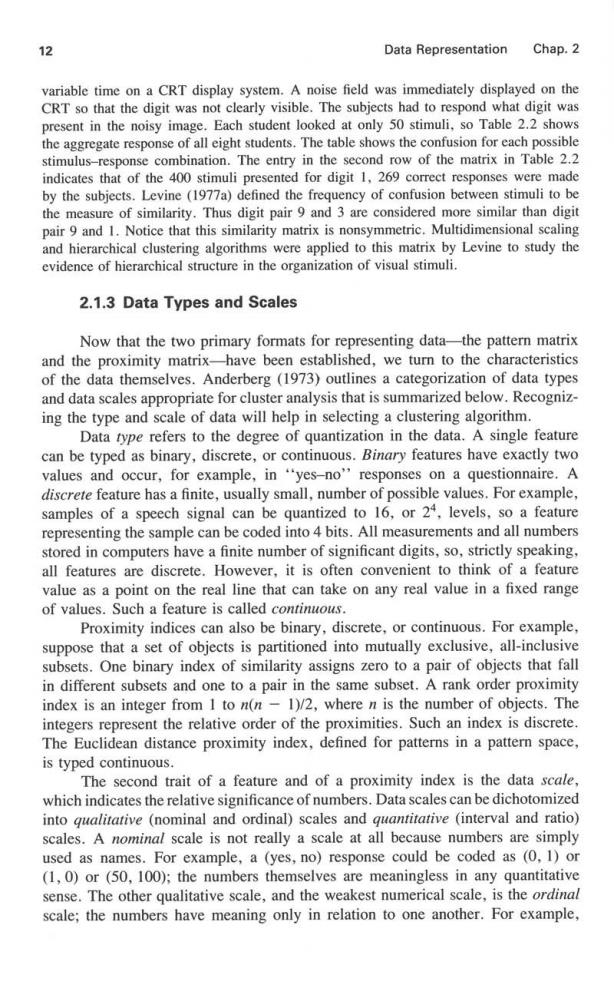
Sec.2.1 Data Types and Data Scales 13 the scales (1,2,3),(10,20,30),and (1,20,300)are all equivalent from an ordinal viewpoint.Binary and discrete features and proximity indices can be coded on these qualitative scales. The separation between numbers has meaning on an interval scale.A unit of measurement exists,and the interpretation of the numbers depends on this unit.For example,a person can be asked to judge satisfaction with politicians on a scale from 0 to 100.The pair of scores (45,55)and the pair (10,90)on two politicians would indicate very different perceptions.Before the number 10 could be interpreted,one would need to know that the scale was 0 to 100 or I to 10 or 10 to 100.Temperature provides another example of an interval scale.A reading of 90 Fahrenheit has a very different implication for comfort than does a temperature of90°Celsius. The strongest scale is the ratio scale,on which numbers have an absolute meaning.This implies that an absolute zero exists along with a unit of measurement, so the ratio between two numbers has meaning.For example,the distance between two cities can be measured in meters,miles,or inches,but doubling the distance always has the same significance when driving from one to the other.Similarly, doubling one's income should double purchasing power,no matter what unit of currency is used.Degrees Kelvin establishes a ratio temperature scale because it has a natural zero.All three data types can be coded on the two quantitative scales. DATA PRESENTATION PATTERN PROXIMITY MATRIX MATRIX Similarity Binary TYPE Discrete TYPE Continuous Dissimilority SCALE SCALE ualitative Nominal Ordinal Interval Ratio Ordinal Interval Rotio Figure 2.2 Formats,types,and scales for data
14 Data Representation Chap.2 Data type and scale are not always of one's choosing.Recognizing type and scale is important in both forming proximity indices and interpreting the results of a cluster analysis.For example,one should realize that human subjects are good at generating binary,qualitative data but that instruments are required to produce continuous,quantitative data.A human subject required to generate discrete, interval data will be under greater stress than one asked to provide binary,ordinal data,so the reliability of data can depend on type and scale.Anderberg(1973) explains conversions from one scale to another.Clustering methods (Chapter 3) use quantitative indices of proximity to assign a cluster label,or name,to each object,so a nominal scale can be generated from a quantitative scale.Multidimen- sional scaling (Section 2.7)changes ordinal scales into ratio scales.The various formats,types,and scales for data are summarized in Figure 2.2. 2.2 PROXIMITY INDICES This section explains some of the more common proximity indices.Anderberg (1973)provides a thorough review of measures of association and their interrelation- ships.A proximity index between the ith and kth patterns is denoted d(i,k)and must satisfy the following three properties: 1.(a)For a dissimilarity:d(i,i)=0,all i (b)For a similarity:d(i,i)max d(i,k),all i 2.d(i,k)=d(k,i),all (i,k) 3.di,k)≥0,all(i,k) Ratio and nominal proximity indices are discussed in separate sections. 2.2.1 Ratio Types A proximity index can be determined in several ways.Suppose that we begin with a pattern matrix [xl,where x is the jth feature for the ith pattern. All features are continuous and measured on a ratio scale.The most common proximity index for such patterns is the Minkowski metric,which measures dissimi- larity.The ith pattern,which is the ith row of the pattern matrix,is denoted by the column vector x;. x=(c1x2,·xd,i=1,2,···,n Here d is the number of features,n the number of patterns,and T denotes vector transpose.The Minkowski metric is defined by d(i,k where r≥I All Minkowski metrics satisfy the additional metric properties stated below. Property 5 is called the triangle inegualiry