Appendix 387 1,3,2.1,320.3 **master element number,number of elements to be defined in the first **row generated including the master element,increment in node numbers **of corresponding nodes from element to element in row (default is 1). **increment in element numbers in row (default is 1),numbers of rows to **be defined(default is 1),increment in node numbers of corresponding **nodes from row to row,increment in element numbers of corresponding **elements from row to row,numbers of layers to be defined(defined is **1),increment in node numbers of corresponding nodes from layer to **layer,increment in element numbers of corresponding elements from **layer to layer *shell section,elset=slab,material=al 1.75.9 **shell thickness,total number of the integration points through its thickness *material,name=al **concrete material parameters definition *elastic 4.15e6,.15 **Young modulus,Poisson ratio *concrete 3000.,0. 5500..0015 **absolute value of compressive stress,absolute value of plastic strain (the **first stress-strain point must be at zero plastic strain and defines the **initial yield point) *failure ratios 1.16,.0836 **ratio of the ultimate biaxial compressive stress to the uniaxial **compressive ultimate stress(default is 1.16),absolute value of the ratio **of uniaxial tensile stress at failure to the uniaxial compressive stress at **failure(default is 0.09),the ratio of the magnitude of a principal **component of plastic strain at ultimate stress in biaxial compression to **the plastic strain at ultimate stress in uniaxial compression,the ratio of **the tensile principal stress value at cracking,in plane stress,when the **other non-zero principal stress component is at the ultimate compressive **stress value,to the tensile cracking stress under uniaxial tension. *tension stiffening **definition of retained tensile stress normal to a crack is a function of the **deformation in the direction of the normal to the crack
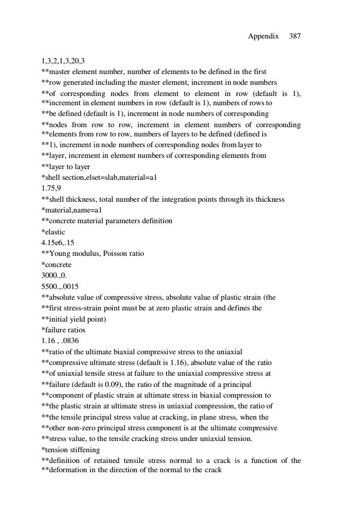
Appendix 387 1,3,2,1,3,20,3 **master element number, number of elements to be defined in the first **row generated including the master element, increment in node numbers **of corresponding nodes from element to element in row (default is 1), **increment in element numbers in row (default is 1), numbers of rows to **be defined (default is 1), increment in node numbers of corresponding **nodes from row to row, increment in element numbers of corresponding **elements from row to row, numbers of layers to be defined (defined is **1), increment in node numbers of corresponding nodes from layer to **layer, increment in element numbers of corresponding elements from **layer to layer *shell section,elset=slab,material=a1 1.75,9 **shell thickness, total number of the integration points through its thickness *material,name=a1 **concrete material parameters definition *elastic 4.15e6,.15 **Young modulus, Poisson ratio *concrete 3000.,0. 5500.,.0015 **absolute value of compressive stress, absolute value of plastic strain (the **first stress-strain point must be at zero plastic strain and defines the **initial yield point) *failure ratios 1.16 , .0836 **ratio of the ultimate biaxial compressive stress to the uniaxial **compressive ultimate stress (default is 1.16), absolute value of the ratio **of uniaxial tensile stress at failure to the uniaxial compressive stress at **failure (default is 0.09), the ratio of the magnitude of a principal **component of plastic strain at ultimate stress in biaxial compression to **the plastic strain at ultimate stress in uniaxial compression, the ratio of **the tensile principal stress value at cracking, in plane stress, when the **other non-zero principal stress component is at the ultimate compressive **stress value, to the tensile cracking stress under uniaxial tension. *tension stiffening **definition of retained tensile stress normal to a crack is a function of the **deformation in the direction of the normal to the crack
388 Random Composites 1.,0. 0.,2.e-3 **fraction of remaining stress to stress at cracking,absolute value of the **direct strain minus the direct strain at cracking *rebar,element=shell,material=slabmt,geometry=isoparametric,name=yy **definition of the rebars,reinforced element type,material name,rebar **geometry type (isoparametric or skew),name of the rebars group slab.014875,1.,-.435,4 **definition of rebars geometry,cross-sectional area of each rebar,spacing **of the rebars in the plane of the shell,position of the rebars in the shell **direction,edge number to which rebar are similar [4] *rebar,element=shell,material=slabmt,geometry=isoparametric,name=xx slab.014875,1.,-.435,1 material.name=slabmt *elastic 29.e6 **Young modulus,Poisson ratio is default *plastic 50.e3 **Yield stress value *boundary **displacement boundary condition definition y-sym,ysymm x-sym,xsymm **symmetry conditions on x-sym,y-sym boundaries 67,3 *restart,write,frequency=999 **option RESTART controls the writing to and reading of the restart file, **which is used by the postprocessor;the option will create a restart **file after each increment at which the increment number is exactly **divisible by N,and at the end of each step of the analysis,regardless of **the value of N at that time *step,inc=30 **option STEP must begin each step definition,parameter INC is equal to **the maximum number of increments in a step(upper bound,the default **value is 10) *static,riks **this option indicates that the step should be analysed as a static load **step:the Riks method is chosen by the RIKS parameter
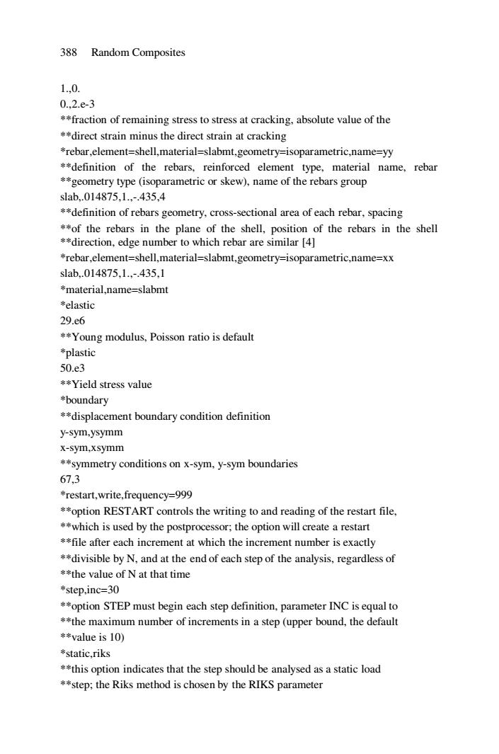
388 Random Composites 1.,0. 0.,2.e-3 **fraction of remaining stress to stress at cracking, absolute value of the **direct strain minus the direct strain at cracking *rebar,element=shell,material=slabmt,geometry=isoparametric,name=yy **definition of the rebars, reinforced element type, material name, rebar **geometry type (isoparametric or skew), name of the rebars group slab,.014875,1.,-.435,4 **definition of rebars geometry, cross-sectional area of each rebar, spacing **of the rebars in the plane of the shell, position of the rebars in the shell **direction, edge number to which rebar are similar [4] *rebar,element=shell,material=slabmt,geometry=isoparametric,name=xx slab,.014875,1.,-.435,1 *material,name=slabmt *elastic 29.e6 **Young modulus, Poisson ratio is default *plastic 50.e3 **Yield stress value *boundary **displacement boundary condition definition y-sym,ysymm x-sym,xsymm **symmetry conditions on x-sym, y-sym boundaries 67,3 *restart,write,frequency=999 **option RESTART controls the writing to and reading of the restart file, **which is used by the postprocessor; the option will create a restart **file after each increment at which the increment number is exactly **divisible by N, and at the end of each step of the analysis, regardless of **the value of N at that time *step,inc=30 **option STEP must begin each step definition, parameter INC is equal to **the maximum number of increments in a step (upper bound, the default **value is 10) *static,riks **this option indicates that the step should be analysed as a static load **step; the Riks method is chosen by the RIKS parameter

Appendix 389 05,1,1,3,-1. **initial time increment,time period of the step,minimum time increment **allowed,maximum increment allowed,maximum value of the load **proportionality factor for the Riks method,node number at which the **value is being monitored,degree of freedom being monitored,value of **the total displacement (or rotation)at the node and degree of freedom **which,if crossed during an increment,ends the step at that increment *cload **concentrated loading definition 1,3,-5000. **node number,number of the corresponding degree of freedom,loading **magnitude in the orientation given by the user by ordering nodes into **shell elements *el print,frequency=10 **option provided tabular printed output of element variables;parameter **FREQUENCY is equal to the output frequency measured in the **increments performed(if this option is omitted,very large printed output **files will be produced by large models in multiple increment analysis!) **all stress components sinv **all stress invariants(MISES,TRESC,PRESS-equivalent pressure stress, **INV3-third stress invariant) c **all strain components pe *all plastic strain component crack **crack orientations in concrete *el file,frequency=10 sinv e pe crack *node file,nset=one **this option allows nodal variables to be written to the ABAQUS results **file (no nodal variables will be written to the results file unless this **option is used!)
Appendix 389 .05,1.,,,,1,3,-1. **initial time increment, time period of the step, minimum time increment **allowed, maximum increment allowed, maximum value of the load **proportionality factor for the Riks method, node number at which the **value is being monitored, degree of freedom being monitored, value of **the total displacement (or rotation) at the node and degree of freedom **which, if crossed during an increment, ends the step at that increment *cload **concentrated loading definition 1,3,-5000. **node number, number of the corresponding degree of freedom, loading **magnitude in the orientation given by the user by ordering nodes into **shell elements *el print,frequency=10 **option provided tabular printed output of element variables; parameter **FREQUENCY is equal to the output frequency measured in the **increments performed (if this option is omitted, very large printed output **files will be produced by large models in multiple increment analysis!) s **all stress components sinv **all stress invariants (MISES,TRESC,PRESS-equivalent pressure stress, **INV3-third stress invariant) e **all strain components pe ** all plastic strain component crack **crack orientations in concrete *el file,frequency=10 s sinv e pe crack *node file,nset=one **this option allows nodal variables to be written to the ABAQUS results **file (no nodal variables will be written to the results file unless this **option is used!)
390 Random Composites 《 *end step **FURTHER COMMENTS **it is possible to provide SHEAR RETENTION parameter to describe the **reduction of the shear modulus as a function of the tensile strain across the **crack;if this parameter is omitted(should be placed after TENSION **STIFFENING lines),it is assumed that the shear retention behaviour depends **only on temperature.EXPANSION parameter may be used to introduce thermal **volume change effects in the concrete.The NLGEOM parameter may be **included in the STEP option when the large strains and rotations associated with **failure of concrete are observed. 8.3 MAPLE Script for Computations of the Homogenised Heat Conductivity Coefficients Mexican hat-Haar basis plot of the input heat conductivity >restart;sig=-.5;k1=0.1;k2:=0.4; kmexh:=2+1/(sqrt(2*Pi)*sig^3)*((exp(-x 2/(2*sig 2)))(x 2/sig 2-1)); >khaar:=piecewise(x<=0.5,k1,x>=0.5,k2); >k:=khaar+0.005*kmexh; plot(k,x=0..1,title='k'); Mexican hat-Haar basis heat conductivity contrast variability restart;sig:=-.5;k1:=contrast"k2;k2:=0.05; kmexh:=2+1/(sqrt(2*Pi)*sig 3)*((exp(-x 2/(2*sig 2)))*(x^2/sig 2-1)); >khaar:=piecewise(x<=0.5,k1,x>=0.5,k2); >k:=khaar+0.005*kmexh; plot3d(k,x=0..1,contrast=5..100,title='k'); Spatial averaging of the Mexican hat-Haar type heat conducitivity >restart;sig:=-.5;k1=0.1;k2:=0.4; kmexh:=2+1/(sqrt(2*Pi)*sig 3)*((exp(-x2/(2*sig2)))*(x 2/sig 2-1)); khaar:=piecewise(x<=0.5,k1,x>=0.5,k2); >k:=khaar+0.005*kmexh; >plot(k,x=0..1,title='k'); >kav:=evalf(int(k,x=0..1)); Classical homogenisation of the Mexican hat-Haar basis type heat conductivity >restart;sig=-.5;k1:=0.1;k2:=0.4;
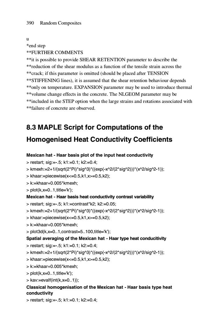
390 Random Composites u *end step **FURTHER COMMENTS **it is possible to provide SHEAR RETENTION parameter to describe the **reduction of the shear modulus as a function of the tensile strain across the **crack; if this parameter is omitted (should be placed after TENSION **STIFFENING lines), it is assumed that the shear retention behaviour depends **only on temperature. EXPANSION parameter may be used to introduce thermal **volume change effects in the concrete. The NLGEOM parameter may be **included in the STEP option when the large strains and rotations associated with **failure of concrete are observed. 8.3 MAPLE Script for Computations of the Homogenised Heat Conductivity Coefficients Mexican hat - Haar basis plot of the input heat conductivity > restart; sig:=-.5; k1:=0.1; k2:=0.4; > kmexh:=2+1/(sqrt(2*Pi)*sig^3)*((exp(-x^2/(2*sig^2)))*(x^2/sig^2-1)); > khaar:=piecewise(x<=0.5,k1,x>=0.5,k2); > k:=khaar+0.005*kmexh; > plot(k,x=0..1,title='k'); Mexican hat - Haar basis heat conductivity contrast variability > restart; sig:=-.5; k1:=contrast*k2; k2:=0.05; > kmexh:=2+1/(sqrt(2*Pi)*sig^3)*((exp(-x^2/(2*sig^2)))*(x^2/sig^2-1)); > khaar:=piecewise(x<=0.5,k1,x>=0.5,k2); > k:=khaar+0.005*kmexh; > plot3d(k,x=0..1,contrast=5..100,title='k'); Spatial averaging of the Mexican hat - Haar type heat conducitivity > restart; sig:=-.5; k1:=0.1; k2:=0.4; > kmexh:=2+1/(sqrt(2*Pi)*sig^3)*((exp(-x^2/(2*sig^2)))*(x^2/sig^2-1)); > khaar:=piecewise(x<=0.5,k1,x>=0.5,k2); > k:=khaar+0.005*kmexh; > plot(k,x=0..1,title='k'); > kav:=evalf(int(k,x=0..1)); Classical homogenisation of the Mexican hat - Haar basis type heat conductivity > restart; sig:=-.5; k1:=0.1; k2:=0.4;
Appendix 391 kmexh:=2+1/(sqrt(2*Pi)*sig^3)*((exp(-x^2/(2*sig 2)))*(x 2/sig 2-1)); >khaar:=piecewise(x<=0.5,k1,x>=0.5,k2); >k:=khaar+0.005*kmexh; >kk:=1/k:kkk:=int(kk,x=0..1):khom:=evalf(1/kkk); Wavelet homogenisation of the Mexican hat-Haar basis type heat conductivity >restart;sig=-.5;k1:=0.1;k2:=0.4; >kmexh:=2+1/(sqrt(2*P1)*sig3)*(exp(-x2/(2*sig2))'(x2/sig2-1): >khaar:=piecewise(x<=0.5,k1,x>=0.5,k2); k:=khaar+0.005*kmexh: >kk:=1/k;kkk:=x/k;kkkk:=1/(2*k); kkk1:=evalf(int(kk,x=0..1));kkk2:=evalf(int(kkk,x=0..1)); kkk3:=evalf(int(kkkk,x=0..1)); khomwav:=evalf(1/(kkk1-2*kkk2+2*kkk3)); Parametric variability of the spatial average of the Mexican hat-Haar type heat conductivity with respect to the contrast and volumetric ratio restart;sig:=-.5;k1:=contrast*k2;k2:=0.05; kmexh:=2+1/(sqrt(2*Pi)*sig 3)*((exp(-x^2/(2*sig 2)))*(x 2/sig 2-1)); khaar:=piecewise(x<=g,k1,x>=g,k2); >k:=khaar+0.005*kmexh; >kav:=evalf(int(k,x=0..1)); >plot3d(kav,contrast=5..100,g=0.1..0.9,title='kav'); Parametric sensitivity of the Mexican hat-Haar basis effective heat conductivity with respect to the contrast and volumetric ratio restart;sig:=-.5;k1:=contrast*k2;k2:=0.05; kmexh:=2+1/(sqrt(2*Pi)*sig 3)*((exp(-x 2/(2*sig 2)))*(x^2/sig 2-1)); khaar:=piecewise(x<=g,k1,x>=g,k2); k:=khaar+0.005*kmexh: >kav:=evalf(int(k,x=0..1)); dkavdcontrast:=diff(kav,contrast)*contrast/kav; >plot3d(dkavdcontrast,contrast=5..100,g=0.1..0.9,title='dkavdcontrast'); dkavdg:=diff(kav,g)"g/kav; >plot3d(dkavdg,contrast=5..100,g=0.1..0.9,title='dkavdg'); Parametric variability of the classically homogenised the Mexican hat-Haar basis heat conductivity with respect to the contrast and volumetric ratio restart;sig:=-.5;k1:=contrast*k2;k2:=0.05; kmexh:=2+1/(sqrt(2*Pi)*sig 3)*((exp(-x 2/(2*sig 2)))*(x^2/sig 2-1)); >khaar:=piecewise(x<g,k1,x>g,k2); >k:=khaar+0.005*kmexh;
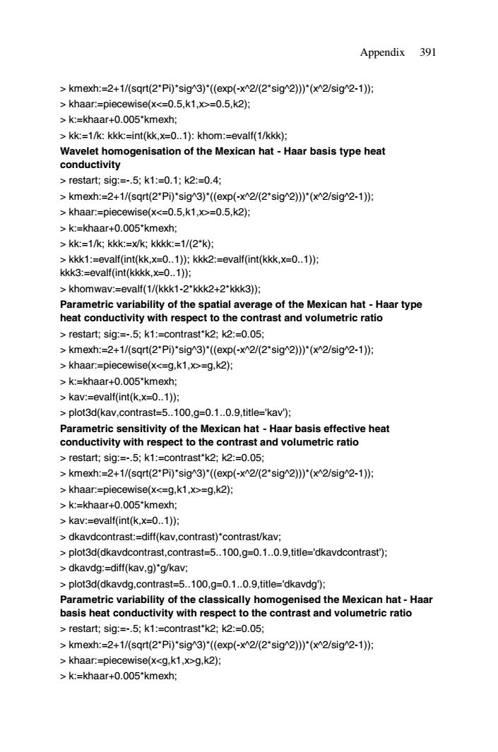
Appendix 391 > kmexh:=2+1/(sqrt(2*Pi)*sig^3)*((exp(-x^2/(2*sig^2)))*(x^2/sig^2-1)); > khaar:=piecewise(x<=0.5,k1,x>=0.5,k2); > k:=khaar+0.005*kmexh; > kk:=1/k: kkk:=int(kk,x=0..1): khom:=evalf(1/kkk); Wavelet homogenisation of the Mexican hat - Haar basis type heat conductivity > restart; sig:=-.5; k1:=0.1; k2:=0.4; > kmexh:=2+1/(sqrt(2*Pi)*sig^3)*((exp(-x^2/(2*sig^2)))*(x^2/sig^2-1)); > khaar:=piecewise(x<=0.5,k1,x>=0.5,k2); > k:=khaar+0.005*kmexh; > kk:=1/k; kkk:=x/k; kkkk:=1/(2*k); > kkk1:=evalf(int(kk,x=0..1)); kkk2:=evalf(int(kkk,x=0..1)); kkk3:=evalf(int(kkkk,x=0..1)); > khomwav:=evalf(1/(kkk1-2*kkk2+2*kkk3)); Parametric variability of the spatial average of the Mexican hat - Haar type heat conductivity with respect to the contrast and volumetric ratio > restart; sig:=-.5; k1:=contrast*k2; k2:=0.05; > kmexh:=2+1/(sqrt(2*Pi)*sig^3)*((exp(-x^2/(2*sig^2)))*(x^2/sig^2-1)); > khaar:=piecewise(x<=g,k1,x>=g,k2); > k:=khaar+0.005*kmexh; > kav:=evalf(int(k,x=0..1)); > plot3d(kav,contrast=5..100,g=0.1..0.9,title='kav'); Parametric sensitivity of the Mexican hat - Haar basis effective heat conductivity with respect to the contrast and volumetric ratio > restart; sig:=-.5; k1:=contrast*k2; k2:=0.05; > kmexh:=2+1/(sqrt(2*Pi)*sig^3)*((exp(-x^2/(2*sig^2)))*(x^2/sig^2-1)); > khaar:=piecewise(x<=g,k1,x>=g,k2); > k:=khaar+0.005*kmexh; > kav:=evalf(int(k,x=0..1)); > dkavdcontrast:=diff(kav,contrast)*contrast/kav; > plot3d(dkavdcontrast,contrast=5..100,g=0.1..0.9,title='dkavdcontrast'); > dkavdg:=diff(kav,g)*g/kav; > plot3d(dkavdg,contrast=5..100,g=0.1..0.9,title='dkavdg'); Parametric variability of the classically homogenised the Mexican hat - Haar basis heat conductivity with respect to the contrast and volumetric ratio > restart; sig:=-.5; k1:=contrast*k2; k2:=0.05; > kmexh:=2+1/(sqrt(2*Pi)*sig^3)*((exp(-x^2/(2*sig^2)))*(x^2/sig^2-1)); > khaar:=piecewise(x<g,k1,x>g,k2); > k:=khaar+0.005*kmexh;