322 Computational Mechanics of Composite Materials e2 0.1+ 0.05 01 0.02 0.04 0.06 008 005 -0.1+ Figure 7.6.Second order wavelet approximation of Young modulus in first scale e3 0.1 0.0吃 0.05 -0.1 Figure 7.7.Third order wavelet approximation of Young modulus in first scale As is shown in the next figures (Figures 7.8 and 7.9),using some special combinations of the basic wavelets (Haar,Mexican hat,Gabor,Morlet,Daubechies and/or sinusoidal waves [323]),the spatial variability of Young modulus for the two component composite with and without some interphase can be computationally simulated using a theoretical description of the spatial distribution of this modulus and the symbolic computation package MAPLE,for instance.For illustration of the problem we consider the Representative Volume Element(RVE) of a two-component composite with the following elastic characteristics: e1=209E9 and e2=209E8 with the RVE length /=1.0 and equal volume fractions of
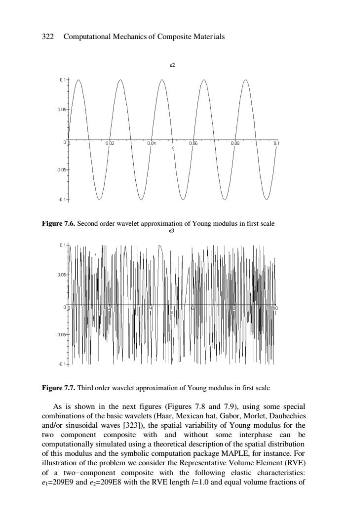
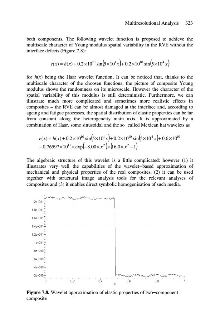
322 Computational Mechanics of Composite Materials Figure 7.6. Second order wavelet approximation of Young modulus in first scale Figure 7.7. Third order wavelet approximation of Young modulus in first scale As is shown in the next figures (Figures 7.8 and 7.9), using some special combinations of the basic wavelets (Haar, Mexican hat, Gabor, Morlet, Daubechies and/or sinusoidal waves [323]), the spatial variability of Young modulus for the two component composite with and without some interphase can be computationally simulated using a theoretical description of the spatial distribution of this modulus and the symbolic computation package MAPLE, for instance. For illustration of the problem we consider the Representative Volume Element (RVE) of a two-component composite with the following elastic characteristics: e1=209E9 and e2=209E8 with the RVE length l=1.0 and equal volume fractions of
Multiresolutional Analysis 323 both components.The following wavelet function is proposed to achieve the multiscale character of Young modulus spatial variability in the RVE without the interface defects (Figure 7.8): e()=h(w)+0.2×100sin5×10'x+0.2x100sin5×104x for h(x)being the Haar wavelet function.It can be noticed that,thanks to the multiscale character of the choosen functions,the picture of composite Young modulus shows the randomness on its microscale.However the character of the spatial variability of this modulus is still deterministic.Furthermore,we can illustrate much more complicated and sometimes more realistic effects in composites-the RVE can be almost damaged at the interface and,according to ageing and fatigue processes,the spatial distribution of elastic properties can be far from constant along the heterogeneity main axis.It is approximated by a combination of Haar,some sinusoidal and the so-called Mexican hat wavelets as e()=h(x)+0.2×100sin5×10'x+0.2x10l0si5×104x+0.6×100 -0.76597×10l×exp8.00×x2kl6.0xx2-1 The algebraic structure of this wavelet is a little complicated:however (1)it illustrates very well the capabilities of the wavelet-based approximation of mechanical and physical properties of the real composites,(2)it can be used together with structural image analysis tools for the relevant analyses of composites and(3)it enables direct symbolic homogenisation of such media. 2e+011 18e+011- 16e+011 14e+011] 12g+011月 1g+011 8e+0101 6e+010- 4e+010月 2e+0101 0.2 04 0.6 5 Figure 7.8.Wavelet approximation of elastic properties of two-component composite
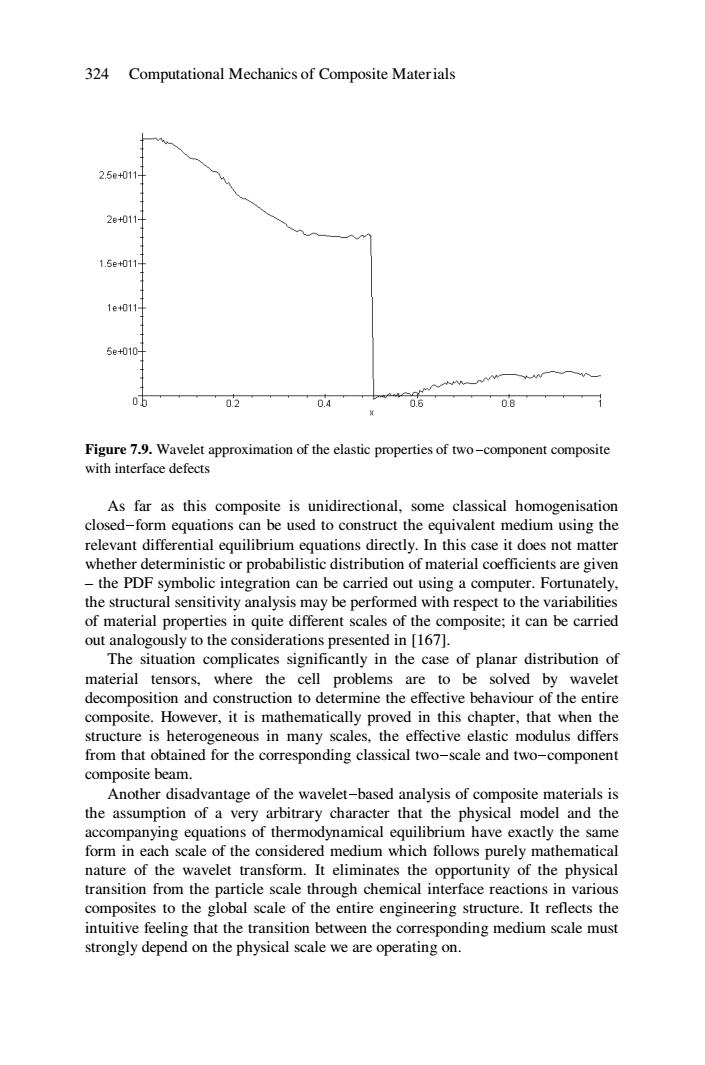
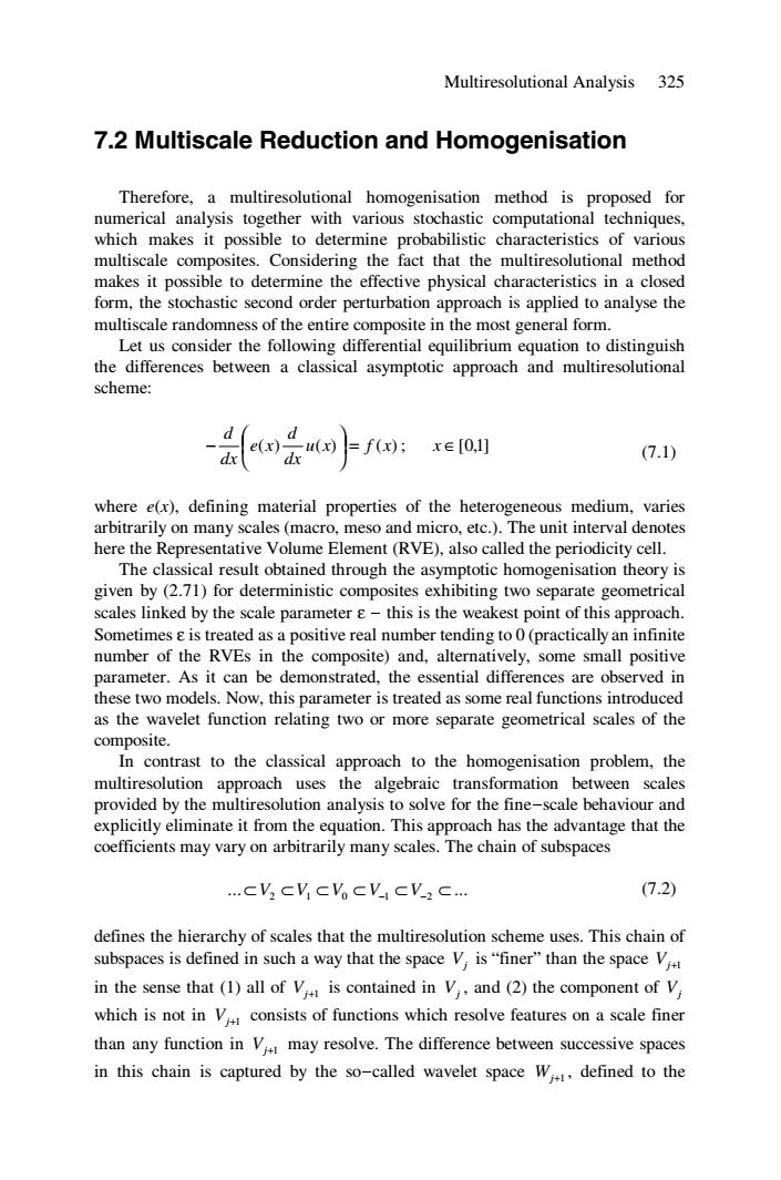
Multiresolutional Analysis 323 both components. The following wavelet function is proposed to achieve the multiscale character of Young modulus spatial variability in the RVE without the interface defects (Figure 7.8): e x h x ( x) ( x) 10 1 10 4 ( ) = ( ) + 0.2×10 sin 5×10 + 0.2×10 sin 5×10 for h(x) being the Haar wavelet function. It can be noticed that, thanks to the multiscale character of the choosen functions, the picture of composite Young modulus shows the randomness on its microscale. However the character of the spatial variability of this modulus is still deterministic. Furthermore, we can illustrate much more complicated and sometimes more realistic effects in composites – the RVE can be almost damaged at the interface and, according to ageing and fatigue processes, the spatial distribution of elastic properties can be far from constant along the heterogeneity main axis. It is approximated by a combination of Haar, some sinusoidal and the so-called Mexican hat wavelets as () ( ) 0.76597 10 exp( )( ) 8.00 16.0 1 ( ) ( ) 0.2 10 sin 5 10 0.2 10 sin 5 10 0.6 10 11 2 2 10 1 10 4 10 − × × − × × × − = + × × + × × + × x x e x h x x x The algebraic structure of this wavelet is a little complicated: however (1) it illustrates very well the capabilities of the wavelet-based approximation of mechanical and physical properties of the real composites, (2) it can be used together with structural image analysis tools for the relevant analyses of composites and (3) it enables direct symbolic homogenisation of such media. Figure 7.8. Wavelet approximation of elastic properties of two-component composite
324 Computational Mechanics of Composite Materials 2.5e+011 2e+011 1.5e+011 1e011 5e+010H 05 02 0.4 0.6 0.8 Figure 7.9.Wavelet approximation of the elastic properties of two-component composite with interface defects As far as this composite is unidirectional,some classical homogenisation closed-form equations can be used to construct the equivalent medium using the relevant differential equilibrium equations directly.In this case it does not matter whether deterministic or probabilistic distribution of material coefficients are given -the PDF symbolic integration can be carried out using a computer.Fortunately, the structural sensitivity analysis may be performed with respect to the variabilities of material properties in quite different scales of the composite;it can be carried out analogously to the considerations presented in [167]. The situation complicates significantly in the case of planar distribution of material tensors,where the cell problems are to be solved by wavelet decomposition and construction to determine the effective behaviour of the entire composite.However,it is mathematically proved in this chapter,that when the structure is heterogeneous in many scales,the effective elastic modulus differs from that obtained for the corresponding classical two-scale and two-component composite beam. Another disadvantage of the wavelet-based analysis of composite materials is the assumption of a very arbitrary character that the physical model and the accompanying equations of thermodynamical equilibrium have exactly the same form in each scale of the considered medium which follows purely mathematical nature of the wavelet transform.It eliminates the opportunity of the physical transition from the particle scale through chemical interface reactions in various composites to the global scale of the entire engineering structure.It reflects the intuitive feeling that the transition between the corresponding medium scale must strongly depend on the physical scale we are operating on
324 Computational Mechanics of Composite Materials Figure 7.9. Wavelet approximation of the elastic properties of two-component composite with interface defects As far as this composite is unidirectional, some classical homogenisation closed-form equations can be used to construct the equivalent medium using the relevant differential equilibrium equations directly. In this case it does not matter whether deterministic or probabilistic distribution of material coefficients are given – the PDF symbolic integration can be carried out using a computer. Fortunately, the structural sensitivity analysis may be performed with respect to the variabilities of material properties in quite different scales of the composite; it can be carried out analogously to the considerations presented in [167]. The situation complicates significantly in the case of planar distribution of material tensors, where the cell problems are to be solved by wavelet decomposition and construction to determine the effective behaviour of the entire composite. However, it is mathematically proved in this chapter, that when the structure is heterogeneous in many scales, the effective elastic modulus differs from that obtained for the corresponding classical two-scale and two-component composite beam. Another disadvantage of the wavelet-based analysis of composite materials is the assumption of a very arbitrary character that the physical model and the accompanying equations of thermodynamical equilibrium have exactly the same form in each scale of the considered medium which follows purely mathematical nature of the wavelet transform. It eliminates the opportunity of the physical transition from the particle scale through chemical interface reactions in various composites to the global scale of the entire engineering structure. It reflects the intuitive feeling that the transition between the corresponding medium scale must strongly depend on the physical scale we are operating on
Multiresolutional Analysis 325 7.2 Multiscale Reduction and Homogenisation Therefore,a multiresolutional homogenisation method is proposed for numerical analysis together with various stochastic computational techniques, which makes it possible to determine probabilistic characteristics of various multiscale composites.Considering the fact that the multiresolutional method makes it possible to determine the effective physical characteristics in a closed form,the stochastic second order perturbation approach is applied to analyse the multiscale randomness of the entire composite in the most general form. Let us consider the following differential equilibrium equation to distinguish the differences between a classical asymptotic approach and multiresolutional scheme: =fx) x∈0,] (7.1) where e(x),defining material properties of the heterogeneous medium,varies arbitrarily on many scales (macro,meso and micro,etc.).The unit interval denotes here the Representative Volume Element(RVE),also called the periodicity cell. The classical result obtained through the asymptotic homogenisation theory is given by (2.71)for deterministic composites exhibiting two separate geometrical scales linked by the scale parameter e-this is the weakest point of this approach. Sometimes e is treated as a positive real number tending to 0(practically an infinite number of the RVEs in the composite)and,alternatively,some small positive parameter.As it can be demonstrated,the essential differences are observed in these two models.Now,this parameter is treated as some real functions introduced as the wavelet function relating two or more separate geometrical scales of the composite. In contrast to the classical approach to the homogenisation problem,the multiresolution approach uses the algebraic transformation between scales provided by the multiresolution analysis to solve for the fine-scale behaviour and explicitly eliminate it from the equation.This approach has the advantage that the coefficients may vary on arbitrarily many scales.The chain of subspaces ...cVCVCVCVCVC... (7.2) defines the hierarchy of scales that the multiresolution scheme uses.This chain of subspaces is defined in such a way that the space V is"finer"than the space V in the sense that (1)all of V is contained in V,,and(2)the component of V which is not in V consists of functions which resolve features on a scale finer than any function in V may resolve.The difference between successive spaces in this chain is captured by the so-called wavelet space W,defined to the
Multiresolutional Analysis 325 7.2 Multiscale Reduction and Homogenisation Therefore, a multiresolutional homogenisation method is proposed for numerical analysis together with various stochastic computational techniques, which makes it possible to determine probabilistic characteristics of various multiscale composites. Considering the fact that the multiresolutional method makes it possible to determine the effective physical characteristics in a closed form, the stochastic second order perturbation approach is applied to analyse the multiscale randomness of the entire composite in the most general form. Let us consider the following differential equilibrium equation to distinguish the differences between a classical asymptotic approach and multiresolutional scheme: ( ) u(x) f (x) dx d e x dx d ⎟ = ⎠ ⎞ ⎜ ⎝ ⎛ − ; ] x ∈[0,1 (7.1) where e(x), defining material properties of the heterogeneous medium, varies arbitrarily on many scales (macro, meso and micro, etc.). The unit interval denotes here the Representative Volume Element (RVE), also called the periodicity cell. The classical result obtained through the asymptotic homogenisation theory is given by (2.71) for deterministic composites exhibiting two separate geometrical scales linked by the scale parameter ε - this is the weakest point of this approach. Sometimes ε is treated as a positive real number tending to 0 (practically an infinite number of the RVEs in the composite) and, alternatively, some small positive parameter. As it can be demonstrated, the essential differences are observed in these two models. Now, this parameter is treated as some real functions introduced as the wavelet function relating two or more separate geometrical scales of the composite. In contrast to the classical approach to the homogenisation problem, the multiresolution approach uses the algebraic transformation between scales provided by the multiresolution analysis to solve for the fine-scale behaviour and explicitly eliminate it from the equation. This approach has the advantage that the coefficients may vary on arbitrarily many scales. The chain of subspaces ... ... ⊂ V2 ⊂V1 ⊂V0 ⊂ V−1 ⊂ V−2 ⊂ (7.2) defines the hierarchy of scales that the multiresolution scheme uses. This chain of subspaces is defined in such a way that the space Vj is “finer” than the space Vj+1 in the sense that (1) all of Vj+1 is contained in Vj , and (2) the component of Vj which is not in Vj+1 consists of functions which resolve features on a scale finer than any function in Vj+1 may resolve. The difference between successive spaces in this chain is captured by the so-called wavelet space Wj+1 , defined to the
326 Computational Mechanics of Composite Materials orthogonal complement of V in V,.An orthogonal basis for the wavelet space Wis constructed which has vanishing moments,i.e.the basis elements are L'-orthogonal to low-degree polynomials.The existence of orthogonal wavelet bases with vanishing moments distinguishes the multiresolution approach from typical multi-scale discretisations provided by finite-element or hierarchical bases.If we are considering a multiresolution analysis defined on a bounded domain,then the hierarchy of scales defined above has the coarsest scale (which is called V),and we write instead VocV1cV-2c.… (7.3) Let us review the multiresolution strategy for the reduction and homogenisation of linear problems.Let us consider to this purpose a bounded linear operator S,:VV,.Since V,is spanned by translations of the function x-k).we know that the operator S,may be written in the form of a matrix.If the multiresolution analysis is defined on a bounded domain,then this matrix is finite; otherwise it is an infinite matrix,which we consider as an operator on L2.Let us consider the equation Six=f (7.4) The decomposition V=VW allows us to split the operator S,into four pieces(recall that W is called the wavelet space and is the"detail"or fine-scale component of V,)and write 色)H) (7.5) where we have A,:W*→W Bg,:V#1→W (7.6) Cs,:Wn→VH T,:V#→V and dd,W.ss,V are the L2-orthogonal projections of x and fonto the W and V spaces.The projection s is thus the coarse-scale component of
326 Computational Mechanics of Composite Materials orthogonal complement of Vj+1 in Vj . An orthogonal basis for the wavelet space Wj+1 is constructed which has vanishing moments, i.e. the basis elements are 2 L -orthogonal to low-degree polynomials. The existence of orthogonal wavelet bases with vanishing moments distinguishes the multiresolution approach from typical multi-scale discretisations provided by finite-element or hierarchical bases. If we are considering a multiresolution analysis defined on a bounded domain, then the hierarchy of scales defined above has the coarsest scale (which is called V0 ), and we write instead ... V0 ⊂ V−1 ⊂ V−2 ⊂ (7.3) Let us review the multiresolution strategy for the reduction and homogenisation of linear problems. Let us consider to this purpose a bounded linear operator S j Vj →Vj : . Since Vj is spanned by translations of the function ( ) x k j φ 2 − , we know that the operator S j may be written in the form of a matrix. If the multiresolution analysis is defined on a bounded domain, then this matrix is finite; otherwise it is an infinite matrix, which we consider as an operator on 2 L . Let us consider the equation S x f j = (7.4) The decomposition Vj =Vj+1 ⊕Wj+1 allows us to split the operator S j into four pieces (recall that Wj+1 is called the wavelet space and is the “detail” or fine-scale component of Vj ) and write ⎟ ⎟ ⎠ ⎞ ⎜ ⎜ ⎝ ⎛ =⎟ ⎟ ⎠ ⎞ ⎜ ⎜ ⎝ ⎛ ⎟ ⎟ ⎠ ⎞ ⎜ ⎜ ⎝ ⎛ f f x x S S S S s d s d C T A B j j j j (7.5) where we have 1 1 1 1 1 1 1 1 : : : : + + + + + + + + → → → → S j j S j j S j j S j j T V V C W V B V W A W W j j j j (7.6) and 1 , dx d y ∈Wj+ , 1 , x y ∈Vj+ s s are the 2 L -orthogonal projections of x and f onto the Wj+1 and Vj+1 spaces. The projection x s is thus the coarse-scale component of