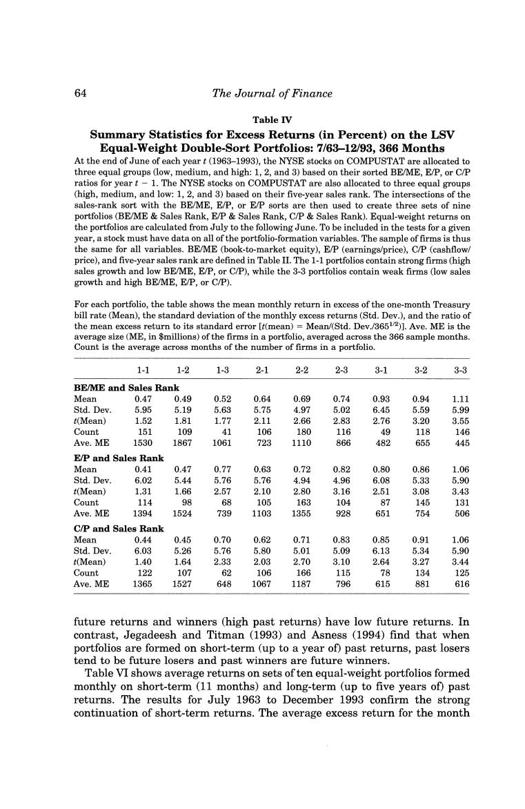
64 The Journal of Finance Table IV Summary Statistics for Excess Returns(in Percent)on the LSV Equal-Weight Double-Sort Portfolios:7/63-12/93,366 Months At the end of June of each yeart(1963-1993),the NYSE stocks on COMPUSTAT are allocated to three equal groups (low,medium,and high:1,2,and 3)based on their sorted BE/ME,E/P,or C/P ratios for year t-1.The NYSE stocks on COMPUSTAT are also allocated to three equal groups (high,medium,and low:1,2,and 3)based on their five-year sales rank.The intersections of the sales-rank sort with the BE/ME,E/P,or E/P sorts are then used to create three sets of nine portfolios (BE/ME Sales Rank,E/P Sales Rank,C/P Sales Rank).Equal-weight returns on the portfolios are calculated from July to the following June.To be included in the tests for a given year,a stock must have data on all of the portfolio-formation variables.The sample of firms is thus the same for all variables.BE/ME (book-to-market equity),E/P (earnings/price),C/P (cashflow/ price),and five-year sales rank are defined in Table II.The 1-1 portfolios contain strong firms(high sales growth and low BE/ME,E/P,or C/P),while the 3-3 portfolios contain weak firms (low sales growth and high BE/ME,E/P,or C/P). For each portfolio,the table shows the mean monthly return in excess of the one-month Treasury bill rate(Mean),the standard deviation of the monthly excess returns(Std.Dev.),and the ratio of the mean excess return to its standard error [t(mean)=Mean/(Std.Dev./3651/2)].Ave.ME is the average size(ME,in $millions)of the firms in a portfolio,averaged across the 366 sample months. Count is the average across months of the number of firms in a portfolio. 1-1 1-2 1-3 2-1 2-2 2-3 3-1 3-2 3-3 BE/ME and Sales Rank Mean 0.47 0.49 0.52 0.64 0.69 0.74 0.93 0.94 1.11 Std.Dev. 5.95 5.19 5.63 5.75 4.97 5.02 6.45 5.59 5.99 t(Mean) 1.52 1.81 1.77 2.11 2.66 2.83 2.76 3.20 3.55 Count 151 109 41 106 180 116 49 118 146 Ave.ME 1530 1867 1061 723 1110 866 482 655 445 E/P and Sales Rank Mean 0.41 0.47 0.77 0.63 0.72 0.82 0.80 0.86 1.06 Std.Dev 6.02 5.44 5.76 5.76 4.94 4.96 6.08 5.33 5.90 t(Mean) 1.31 1.66 2.57 2.10 2.80 3.16 2.51 3.08 3.43 Count 114 98 68 105 163 104 87 145 131 Ave.ME 1394 1524 739 1103 1355 928 651 754 506 C/P and Sales Rank Mean 0.44 0.45 0.70 0.62 0.71 0.83 0.85 0.91 1.06 Std.Dev 6.03 5.26 5.76 5.80 5.01 5.09 6.13 5.34 5.90 t(Mean) 1.40 1.64 2.33 2.03 2.70 3.10 2.64 3.27 3.44 Count 122 107 62 106 166 115 78 134 125 Ave.ME 1365 1527 648 1067 1187 796 615 881 616 future returns and winners(high past returns)have low future returns.In contrast,Jegadeesh and Titman (1993)and Asness (1994)find that when portfolios are formed on short-term (up to a year of)past returns,past losers tend to be future losers and past winners are future winners. Table VI shows average returns on sets of ten equal-weight portfolios formed monthly on short-term (11 months)and long-term (up to five years of)past returns.The results for July 1963 to December 1993 confirm the strong continuation of short-term returns.The average excess return for the month
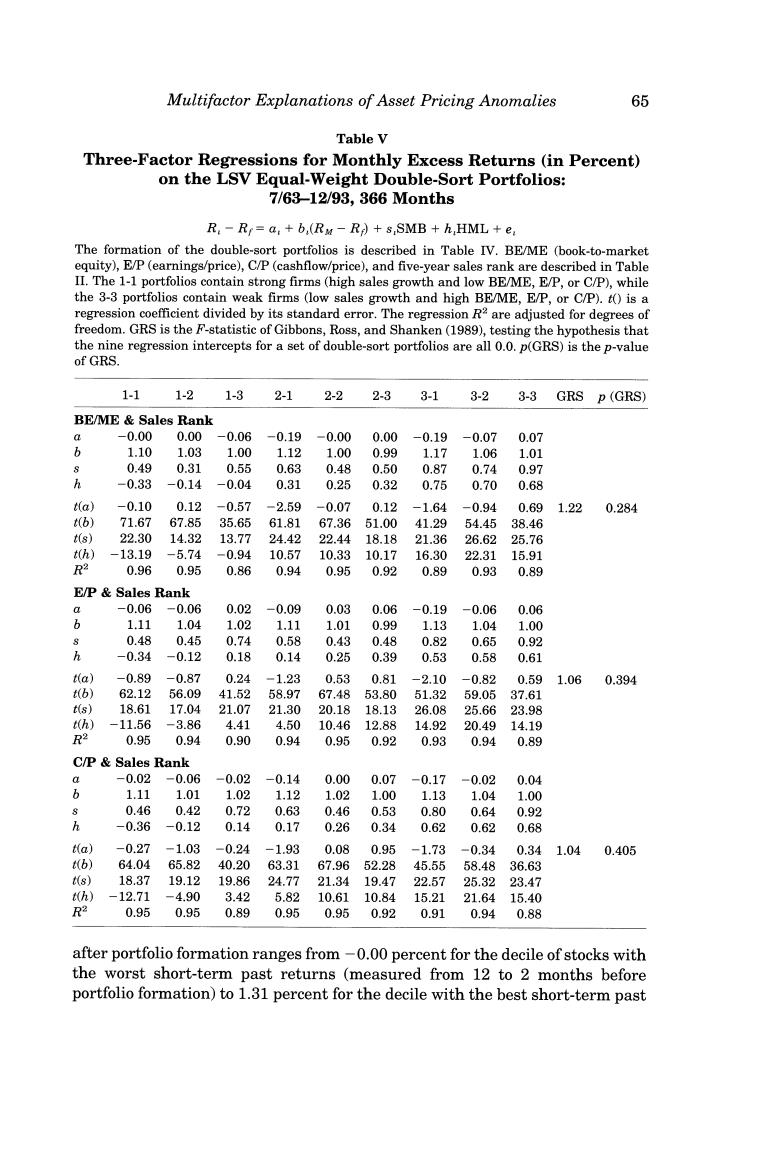
Multifactor Explanations of Asset Pricing Anomalies 65 Table V Three-Factor Regressions for Monthly Excess Returns (in Percent) on the LSV Equal-Weight Double-Sort Portfolios: 7/63-12/93,366 Months R.-R=a +6,(Ry-R s SMB hHML +e The formation of the double-sort portfolios is described in Table IV.BE/ME (book-to-market equity),E/P(earnings/price),C/P(cashflow/price),and five-year sales rank are described in Table II.The 1-1 portfolios contain strong firms (high sales growth and low BE/ME,E/P,or C/P),while the 3-3 portfolios contain weak firms (low sales growth and high BE/ME,E/P,or C/P).t()is a regression coefficient divided by its standard error.The regression R2 are adjusted for degrees of freedom.GRS is the F-statistic of Gibbons,Ross,and Shanken(1989),testing the hypothesis that the nine regression intercepts for a set of double-sort portfolios are all 0.0.p(GRS)is the p-value of GRS. 1-1 1-2 1-3 2-1 2-2 2-3 3-1 3-2 3-3 GRS D(GRS) BE/ME Sales Rank -0.00 0.00 -0.06 -0.19 -0.00 0.00 -0.19 -0.07 0.07 b 1.10 1.03 1.00 1.12 1.00 0.99 1.17 1.06 1.01 0.49 0.31 0.55 0.63 0.48 0.50 0.87 0.74 0.97 -0.33 -0.14 -0.04 0.31 0.25 0.32 0.75 0.70 0.68 ta) -0.10 0.12 -0.57 -2.59 -0.07 0.12 -1.64 -0.94 0.69 1.22 0.284 t(b) 71.67 67.85 35.65 61.81 67.3651.00 41.29 54.45 38.46 t(s) 22.30 14.32 13.77 24.42 22.44 18.18 21.36 26.62 25.76 t(h) -13.19 -5.74 -0.94 10.57 10.33 10.17 16.30 22.31 15.91 R2 0.96 0.95 0.86 0.94 0.95 0.92 0.89 0.93 0.89 E/P Sales Rank a -0.06-0.06 0.02 -0.09 0.03 0.06 -0.19 -0.06 0.06 6 1.11 1.04 1.02 1.11 1.01 0.99 1.13 1.04 1.00 0.48 0.45 0.74 0.58 0.43 0.48 0.82 0.65 0.92 -0.34 -0.12 0.18 0.14 0.25 0.39 0.53 0.58 0.61 t(a) -0.89 -0.87 0.24 -1.23 0.53 0.81 -2.10 -0.82 0.59 1.060.394 tb)】 62.12 56.09 41.52 58.97 67.48 53.80 51.32 59.0537.61 t(s) 18.61 17.04 21.07 21.30 20.18 18.13 26.08 25.66 23.98 (h) -11.56 -3.86 4.41 4.50 10.46 12.88 14.92 20.49 14.19 R2 0.95 0.94 0.90 0.94 0.95 0.92 0.93 0.94 0.89 C/P Sales Rank a -0.02 -0.06 -0.02 -0.14 0.00 0.07 -0.17 -0.02 0.04 b 1.11 1.01 1.02 1.12 1.02 1.00 1.13 1.04 1.00 0.46 0.42 0.72 0.63 0.46 0.53 0.80 0.64 0.92 公 -0.36 -0.12 0.14 0.17 0.26 0.34 0.62 0.62 0.68 Ha) -0.27 -1.03 -0.24 -1.93 0.08 0.95 -1.73-0.34 0.34 1.040.405 t(b) 64.04 65.82 40.2063.3167.9652.28 45.55 58.4836.63 t(s) 18.37 19.12 19.8624.77 21.34 19.47 22.57 25.3223.47 t(h) -12.71 -4.90 3.42 5.8210.61 10.8415.21 21.6415.40 R2 0.950.95 0.890.950.950.920.910.940.88 after portfolio formation ranges from-0.00 percent for the decile of stocks with the worst short-term past returns (measured from 12 to 2 months before portfolio formation)to 1.31 percent for the decile with the best short-term past