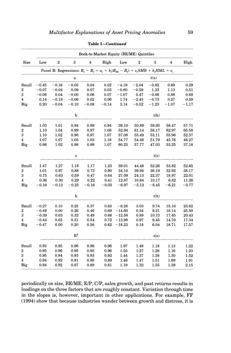
Multifactor Explanations of Asset Pricing Anomalies 59 Table I-Continued Book-to-Market Equity (BE/ME)Quintiles Size Low 2 3 4 High Low 2 3 4 High Panel B:Regressions:R:-Rr=a;+b (RM -R)+s,SMB +h HML +e 9 t(a) Small -0.45 -0.16 -0.05 0.04 0.02 -4.19 -2.04 -0.82 0.69 0.29 2 -0.07 -0.04 0.09 0.07 0.03 -0.80 -0.59 1.33 1.13 0.51 3 -0.08 0.04 -0.00 0.06 0.07 -1.07 0.47 -0.06 0.88 0.89 4 0.14 -0.19 -0.06 0.02 0.06 1.74 -2.43 -0.73 0.27 0.59 Big 0.20 -0.04 -0.10 -0.08 -0.14 3.14 -0.52 -1.23 -1.07 -1.17 b t(b) Small 1.03 1.01 0.94 0.89 0.94 39.10 50.89 59.93 58.47 57.71 2 1.10 1.04 0.99 0.97 1.08 52.94 61.14 58.17 62.97 65.58 3 1.10 1.02 0.98 0.97 1.07 57.08 55.49 53.11 55.96 52.37 4 1.07 1.07 1.05 1.03 1.18 54.77 54.48 51.79 45.76 46.27 Big 0.96 1.02 0.98 0.99 1.07 60.25 57.77 47.03 53.25 37.18 t(s) Small 1.47 1.27 1.18 1.17 1.23 39.01 44.48 52.26 53.82 52.65 2 1.01 0.97 0.88 0.73 0.90 34.10 39.94 36.19 32.92 38.17 3 0.75 0.63 0.59 0.47 0.64 27.09 24.13 22.37 18.97 22.01 4 0.36 0.30 0.29 0.22 0.41 12.87 10.64 10.17 6.82 11.26 Big -0.16 -0.13 -0.25 -0.16 -0.03 -6.97 -5.12 -8.45 -6.21 -0.77 h t(h) Smal1-0.27 0.10 0.25 0.37 0.63 -6.28 3.03 9.74 15.16 23.62 2 -0.49 0.00 0.26 0.46 0.69 -14.66 0.34 9.21 18.14 25.59 3 -0.39 0.03 0.32 0.49 0.68 -12.56 0.89 10.73 17.45 20.43 4 -0.44 0.03 0.31 0.54 0.72 -13.98 0.97 9.45 14.70 17.34 Big -0.47 0.00 0.20 0.56 0.82 -18.23 0.18 6.04 18.71 17.57 R2 s(e) Small 0.93 0.95 0.96 0.96 0.96 1.97 1.49 1.18 1.13 1.22 2 0.95 0.96 0.95 0.95 0.96 1.55 1.27 1.28 1.16 1.23 3 0.95 0.94 0.93 0.93 0.92 1.44 1.37 1.38 1.30 1.52 4 0.94 0.92 0.91 0.88 0.89 1.46 1.47 1.51 1.69 1.91 Big 0.94 0.92 0.87 0.89 0.81 1.19 1.32 1.55 1.39 2.15 periodically on size,BE/ME,E/P,C/P,sales growth,and past returns results in loadings on the three factors that are roughly constant.Variation through time in the slopes is,however,important in other applications.For example,FF (1994)show that because industries wander between growth and distress,it is
60 The Journal of Finance critical to allow for variation in SMB and HML slopes when applying (1)and (2)to industries. II.LSV Deciles Lakonishok,Shleifer,and Vishny(LSV 1994)examine the returns on sets of deciles formed from sorts on BE/ME,E/P,C/P,and five-year sales rank.Table II summarizes the excess returns on our versions of these portfolios.The portfolios are formed each year as in LSV using COMPUSTAT accounting data for the fiscal year ending in the current calendar year(see table footnote).We then calculate returns beginning in July of the following year.(LSV start their returns in April.)To reduce the influence of small stocks in these (equal- weight)portfolios,we use only NYSE stocks.(LSV use NYSE and AMEX.)To be included in the tests for a given year,a stock must have data on all the LSV variables.Thus,firms must have COMPUSTAT data on sales for six years before they are included in the return tests.As in LSV,this reduces biases that might arise because COMPUSTAT includes historical data when it adds firms (Banz and Breen (1986),Kothari,Shanken,and Sloan(1995)). Our sorts of NYSE stocks in Table II produce strong positive relations between average return and BE/ME,E/P,or C/P,much like those reported by LSV for NYSE and AMEX firms.Like LSV,we find that past sales growth is negatively related to future return.The estimates of the three-factor regres- sion (2)in Table III show,however,that the three-factor model (1)captures these patterns in average returns.The regression intercepts are consistently small.Despite the strong explanatory power of the regressions(most R2 values are greater than 0.92),the GRS tests never come close to rejecting the hypoth- esis that the three-factor model describes average returns.In terms of both the magnitudes of the intercepts and the GRS tests,the three-factor model does a better job on the LSV deciles than it does on the 25 FF size-BE/ME portfolios. (Compare Tables I and III.) For perspective on why the three-factor model works so well on the LSV portfolios,Table III shows the regression slopes for the C/P deciles.Higher-C/P portfolios produce larger slopes on SMB and especially HML.This pattern in the slopes is also observed for the BE/ME and E/P deciles(not shown).It seems that dividing an accounting variable by stock price produces a characterization of stocks that is related to their loadings on HML.Given the evidence in FF (1995)that loadings on HML proxy for relative distress,we can infer that low BE/ME,E/P,and C/P are typical of strong stocks,while high BE/ME,E/P,and C/P are typical of stocks that are relatively distressed.The patterns in the loadings of the BE/ME,E/P,and C/P deciles on HML,and the high average value of HML(0.46 percent per month,6.33 percent per year)largely explain how the three-factor regressions transform the strong positive relations be- tween average return and these ratios(Table II)into intercepts that are close to0.0. Among the sorts in Table III,the three-factor model has the hardest time with the returns on the sales-rank portfolios.Recall that high sales-rank firms

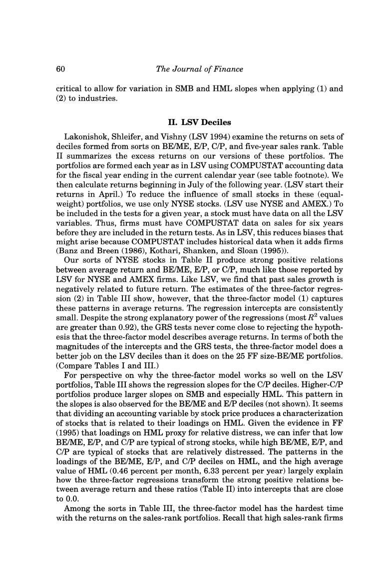
Multifactor Explanations of Asset Pricing Anomalies 61 Table II Summary Statistics for Simple Monthly Excess Returns(in Percent) on the LSV Equal-Weight Deciles:7/63-12/93,366 Months At the end of June of each yeart(1963-1993),the NYSE stocks on COMPUSTAT are allocated to ten portfolios,based on the decile breakpoints for BE/ME(book-to-market equity),E/P (earnings/price),C/P(cashflow/price),and past five-year sales rank(5-Yr SR).Equal-weight returns on the portfolios are calculated from July to the following June,resulting in a time series of 366 monthly returns for July 1963 to December 1993.To be included in the tests for a given year,a stock must have data on all of the portfolio-formation variables of this table. Thus,the sample of firms is the same for all variables. For portfolios formed in June of year t,the denominator of BE/ME,E/P,and C/P is market equity (ME,stock price times shares outstanding)for the end of December of year t-1,and BE,E,and C are for the fiscal year ending in calendar year t-1.Book equity BE is defined in Table I.E is earnings before extraordinary items but after interest,depreciation,taxes,and preferred divi- dends.Cash flow,C,is E plus depreciation. The five-year sales rank for June of year t,5-Yr SR(t),is the weighted average of the annual sales growth ranks for the prior five years,that is, 5 5-Yr SR(t)=> (6-j)×Rank(t-j) 1=1 The sales growth for year t-j is the percentage change in sales from t-j-1 to t-j, In[Sales(t-j)/Sales(t-j-1)].Only firms with data for all five prior years are used to determine the annual sales growth ranks for years t-5 to t-1. For each portfolio,the table shows the mean monthly return in excess of the one-month Treasury bill rate (Mean),the standard deviation of the monthly excess returns(Std.Dev.),and the ratio of the mean excess return to its standard error [t(mean)=Mean/(Std.Dev./36512)].Ave ME is the average size(ME,in $millions)of the firms in a portfolio,averaged across the 366 sample months. Deciles 1 2 3 4 5 6 9 10 BEME Low High Mean 0.42 0.50 0.53 0.58 0.65 0.72 0.81 0.84 1.03 1.22 Std.Dev. 5.81 5.56 5.57 5.52 5.23 5.03 4.96 5.06 5.52 6.82 t(Mean) 1.39 1.72 1.82 2.02 2.38 2.74 3.10 3.17 3.55 3.43 Ave.ME 2256 1390 1125 1037 1001 864 838 730 572 362 EP Low High Mean 0.55 0.45 0.54 0.63 0.67 0.77 0.82 0.90 0.99 1.03 Std.Dev. 6.09 5.62 5.51 5.35 5.14 5.18 4.94 4.88 5.05 5.87 t(Mean) 1.72 1.52 1.89 2.24 2.49 2.84 3.16 3.51 3.74 3.37 Ave.ME 1294 1367 1211 1209 1411 1029 1022 909 862 661 C/P Low High Mean 0.43 0.45 0.60 0.67 0.70 0.76 0.77 0.86 0.97 1.16 Std.Dev. 5.80 5.67 5.57 5.39 5.39 5.19 5.00 4.88 4.96 6.36 t(Mean) 1.41 1.52 2.06 2.37 2.47 2.78 2.93 3.36 3.75 3.47 Ave.ME 1491 1266 1112 1198 990 994 974 951 990 652 5-Yr SR High Low Mean 0.47 0.63 0.70 0.68 0.67 0.74 0.70 0.78 0.89 1.03 Std.Dev. 6.39 5.66 5.46 5.15 5.22 5.10 5.00 5.10 5.25 6.13 t(Mean) 1.42 2.14 2.45 2.52 2.46 2.78 2.68 2.91 3.23 3.21 Ave.ME 937 1233 1075 1182 1265 1186 1075 884 744 434
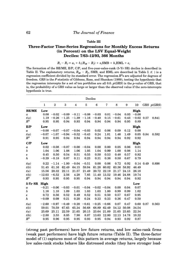
62 The Journal of Finance Table IⅡ Three-Factor Time-Series Regressions for Monthly Excess Returns (in Percent)on the LSV Equal-Weight Deciles:7/63-12/93,366 Months Ri-R=ai+b:(RM-R+s SMB+h;HML+e; The formation of the BE/ME,E/P,C/P,and five-year-sales-rank (5-Yr SR)deciles is described in Table II.The explanatory returns,R-R,SMB,and HML are described in Table I.t()is a regression coefficient divided by its standard error.The regression R2s are adjusted for degrees of freedom.GRS is the F-statistic of Gibbons,Ross,and Shanken(1989),testing the hypothesis that the regression intercepts for a set of ten portfolios are all 0.0.p(GRS)is the p-value of GRS,that is,the probability of a GRS value as large or larger than the observed value if the zero-intercepts hypothesis is true. Deciles 1 3 4 5 6 7 8 9 10 GRS D(GRS) BE/ME Low High 令 0.08 -0.02 -0.09 -0.11-0.08 -0.03 0.01-0.040.03 -0.00 ) 1.19 -0.26 -1.25 -1.39 -1.16-0.40 0.15-0.61 0.43 -0.020.570.841 R2 0.95 0.95 0.94 0.93 0.940.94 0.940.940.95 0.89 EP Low High a -0.00-0.07 -0.07-0.04-0.03 0.020.06 0.090.12 0.00 ta) -0.07-1.07 -0.94-0.52-0.43 0.241.01 1.461.49 0.050.840.592 R2 0.91 0.95 0.94 0.94 0.94 0.940.94 0.940.92 0.92 C/P Low High 0.02-0.08 -0.07-0.00 -0.04 0.000.00 0.050.060.01 b 1.04 1.06 1.08 1.06 1.05 1.04 0.99 1.000.98 1.14 0.45 0.50 0.54 0.51 0.55 0.50 0.53 0.48 0.57 0.92 b -0.39-0.18 0.07 0.11 0.23 0.310.36 0.500.67 0.79 t(a) 0.22-1.14-1.00 -0.04 -0.51 0.00 0.06 0.720.92 0.140.49 0.898 t(b) 51.4561.1662.4964.1559.04 61.2860.0263.3658.92 46.49 t(s) 15.5620.3222.1121.5721.4920.7222.1921.1724.1326.18 t(h) -12.03 -6.52 2.564.28 7.8511.4013.5219.4624.8819.74 R2 0.93 0.95 0.95 0.95 0.94 0.940.94 0.940.94 0.92 5-Yr SR High Low -0.21 -0.06 -0.03-0.01 -0.04 -0.02-0.04 0.000.04 0.07 6 1.16 1.10 1.09 1.03 1.03 1.031.00 0.99 0.99 1.02 0.72 0.56 0.52 0.49 0.52 0.510.500.570.67 0.95 h -0.09 0.09 0.21 0.20 0.24 0.330.33 0.36 0.47 0.50 t(a) -2.60-0.97-0.49-0.20-0.61-0.25-0.660.070.47 0.600.870.563 t(b) 59.0170.5967.6565.3456.6868.8962.4954.1250.0834.54 t(s) 25.6925.1122.5921.6520.1523.6421.8921.6523.6522.34 t(h) -2.88 3.55 8.057.98 8.0713.6312.8012.1314.7810.32 R2 0.950.960.950.950.930.950.940.930.920.87 (strong past performers)have low future returns,and low sales-rank firms (weak past performers)have high future returns(Table II).The three-factor model of(1)captures most of this pattern in average returns,largely because low sales-rank stocks behave like distressed stocks (they have stronger load-
Multifactor Explanations of Asset Pricing Anomalies 63 ings on HML).But a hint of the pattern is left in the regression intercepts. Except for the highest sales-rank decile,however,the intercepts are close to 0.0.Moreover,although the intercepts for the sales-rank deciles produce the largest GRS F-statistic(0.87),it is close to the median of its distribution when the true intercepts are all 0.0(its p-value is 0.563).This evidence that the three-factor model describes the returns on the sales-rank deciles is important since sales rank is the only portfolio-formation variable (here and in LSV)that is not a transformed version of stock price.(See also the industry tests in FF (1994).) III.LSV Double-Sort Portfolios LSV argue that sorting stocks on two accounting variables more accurately distinguishes between strong and distressed stocks,and produces larger spreads in average returns.Because accounting ratios with stock price in the denominator tend to be correlated,LSV suggest combining sorts on sales rank with sorts on BE/ME,E/P,or C/P.We follow their procedure and separately sort firms each year into three groups (low 30 percent,medium 40 percent,and high 30 percent)on each variable.We then form sets of nine portfolios as the intersections of the sales-rank sort and the sorts on BE/ME,E/P,or C/P. Confirming their results,Table IV shows that the sales-rank sort increases the spread of average returns provided by the sorts on BE/ME,E/P,or C/P.In fact, the two double-whammy portfolios,combining low BE/ME,E/P,or C/P with high sales growth (portfolio 1-1),and high BE/ME,E/P,or C/P with low sales growth(portfolio 3-3),always have the lowest and highest post-formation average returns. Table V shows that the three-factor model has little trouble describing the returns on the LSV double-sort portfolios.Strong negative loadings on HML (which has a high average premium)bring the low returns on the 1-1 portfolios comfortably within the predictions of the three-factor model;the most extreme intercept for the 1-1 portfolios is-6 basis points (-0.06 percent)per month and less than one standard error from 0.0.Conversely,because the 3-3 port- folios have strong positive loadings on SMB and HML (they behave like smaller distressed stocks),their high average returns are also predicted by the three-factor model.The intercepts for these portfolios are positive,but again quite close to (less than 8 basis points and 0.7 standard errors from)0.0. The GRS tests in Table V support the inference that the intercepts in the three-factor regression(2)are 0.0;the smallest p-value is 0.284.Thus,whether the spreads in average returns on the LSV double-sort portfolios are caused by risk or over-reaction,the three-factor model in equation (1)describes them parsimoniously. IV.Portfolios Formed on Past Returns DeBondt and Thaler (1985)find that when portfolios are formed on long- term (three-to five-year)past returns,losers (low past returns)have high