12 Abstract Data Types and Algorithms Each Sr is a simple assignment.The asymptotic time complexity of this state- ment can now be determined using the above rules. Time for each SI:O(1) Time for begin S1;S2;S3;S4 end;:O(1)+O(1)+O(1)+O(1)=O(1) Time for the inner loop:I.O(1)=O(D.0(1)=0(1.I)=O(I) Time for the outer loop-∑O① I=1 =0(1/2n2+1/2n) =0(1/2n2) =0(n2) Therefore,the whole statement has asymptotic time complexity O(n2).The Big O notation enables us to define an upper bound for the growth rate of time complexity of an algorithm.To find a lower bound for time complexity,we define Big as: T(n)=(f(n))if there exists a constant Csuch that T(n)>Cf(n) for infinitely many n The reason that Big is defined for infinitely many n and not for all n greater than a given number is that many algorithms are very fast on some sizes of input but not all.For example 2n n is odd T(n)= 3n2-10 n is even Tm)≥n2n=4,6,8,. Therefore T(n)=(n2). 1.4 Importance of Growth Rate of Time Complexities One might reason that,since computing times are steadily decreasing,we do not have to worry so much about developing efficient algorithms to solve problems. We can simply run our programs on a more advanced computer.Unfortunately, this does not work in practice for two reasons.Firstly,computers tend to be presented with more and more sophisticated instances of a problem and it may not be practical to keep on moving to more advanced machines (faster).Secondly, and more importantly,the growth rate of the time complexity of an algorithm is the limiting factor which determines if larger problems can be solved in a reasonable amount of time.To clarify this point,let us consider six algorithms A1,A2,...,A6 and observe their behaviour as they are run on two computers;
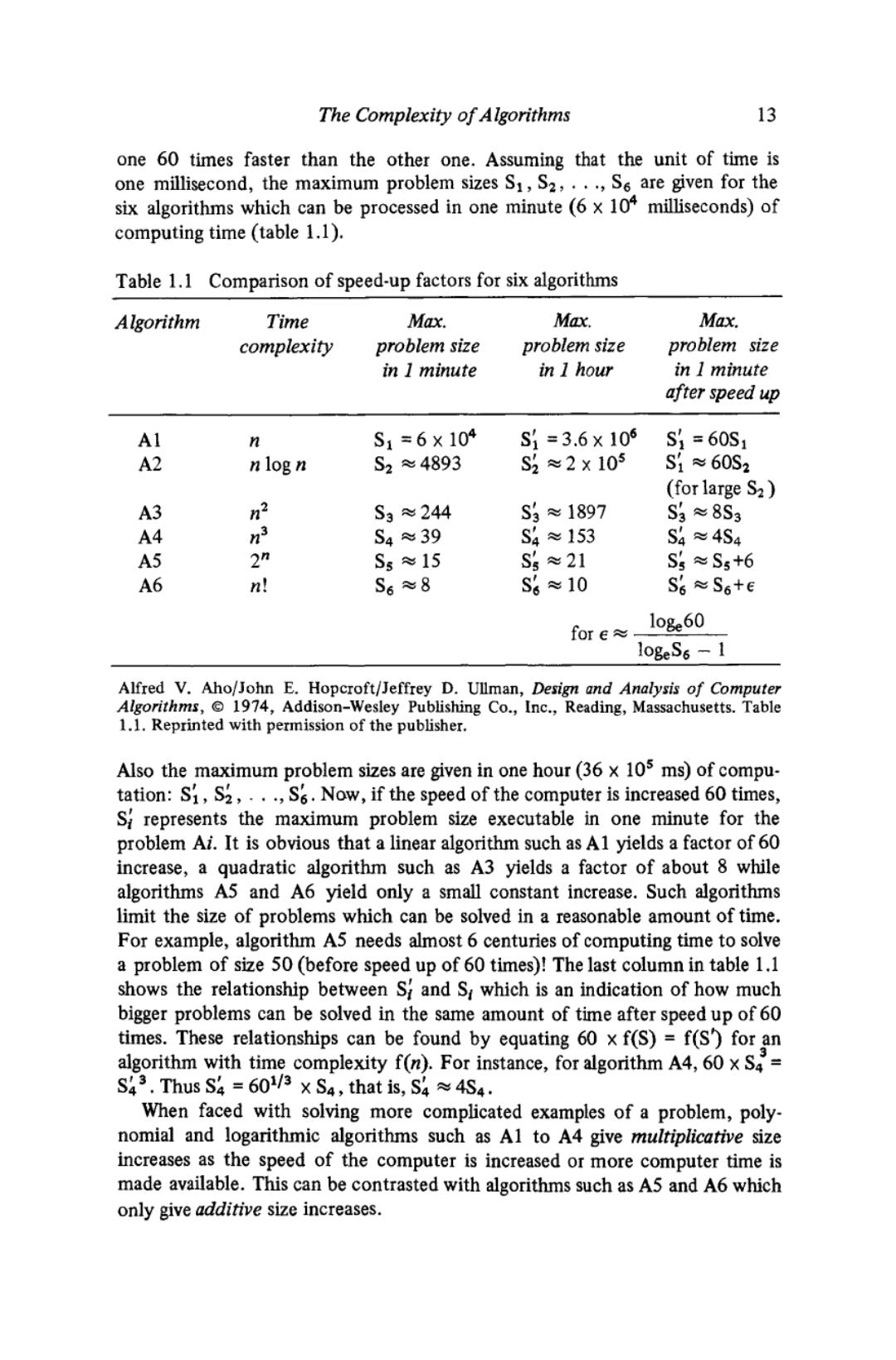
The Complexity of Algorithms 13 one 60 times faster than the other one.Assuming that the unit of time is one millisecond,the maximum problem sizes S1,S2,...,S6 are given for the six algorithms which can be processed in one minute (6 x 10⁴ milliseconds)of computing time (table 1.1). Table 1.1 Comparison of speed-up factors for six algorithms Algorithm Time Max. Max. Max. complexity problem size problem size problem size in I minute in 1 hour in I minute after speed up Al n S1=6×10⁴ S1=3.6×10⁶ S1=60S1 A2 nlog n S2≈4893 S2≈2x10⁵ S1≈60S2 (for large S2) A3 n2 S3≈244 S3≈1897 Sg≈8S3 A4 S4≈39 S4≈153 S4≈4S4 A5 2 Ss≈15 S%≈21 Sg≈S5+6 A6 n! S6≈8 S%≈10 S6≈S6+e fore≈ loge60 logeS6 -1 Alfred V.Aho/John E.Hopcroft/Jeffrey D.Ullman,Design and Analysis of Computer Algorithms,1974,Addison-Wesley Publishing Co.,Inc.,Reading,Massachusetts.Table 1.1.Reprinted with permission of the publisher. Also the maximum problem sizes are given in one hour(36 x 105 ms)of compu- tation:S1,S2,...,S.Now,if the speed of the computer is increased 60 times, Srepresents the maximum problem size executable in one minute for the problem Ai.It is obvious that a linear algorithm such as Al yields a factor of 60 increase,a quadratic algorithm such as A3 yields a factor of about 8 while algorithms A5 and A6 yield only a small constant increase.Such algorithms limit the size of problems which can be solved in a reasonable amount of time. For example,algorithm A5 needs almost 6 centuries of computing time to solve a problem of size 50(before speed up of 60 times)!The last column in table 1.1 shows the relationship between S and S which is an indication of how much bigger problems can be solved in the same amount of time after speed up of 60 times.These relationships can be found by equating 60 x f(S)=f(S)for an algorithm with time complexity f(n).For instance,for algorithm A4,60 x S4= S43.Thus S4=60/3×S4,that is,S4≈4S4. When faced with solving more complicated examples of a problem,poly- nomial and logarithmic algorithms such as Al to A4 give multiplicative size increases as the speed of the computer is increased or more computer time is made available.This can be contrasted with algorithms such as A5 and A6 which only give additive size increases
14 Abstract Data Types and Algorithms So it can be seen that asymptotically efficient algorithms are those which have polynomial or logarithmic time complexities.These are known as poly- nomial algorithms,since they can be bounded by a polynomial;that is,there exists a polynomial P(n)such that f(n)s CP(n)for all n>no where C and no are two constants and f(n)is the time complexity of the algorithm.For instance, A2 is a polynomial algorithm since log n sn for all n>1.Algorithms which are not polynomial are called exponential.Algorithms A5 and A6 are exponen- tial.Almost all the algorithms described in this book are polynomial algorithms. Certain classes of problems may only have exponential algorithms.Such prob- lems are classified as very hard problems.These and some techniques for deriving good algorithms for them are discussed in chapter 12.The spectrum of algorithm complexity can be illustrated as follows: 1<loglog n<logn<n<n logn <n2<n3 <...<2n <n! Note that although an exponential algorithm is asymptotically worse than a poly- nomial one,it may however,for small values of n,be a better algorithm.For instance,2n 100n2 for n=1,2,...,13,14.So for small n,it may be best to use an exponential algorithm.Also,if an algorithm is to be executed only a few times,the efforts to find an efficient algorithm may not be justified and hence a slower algorithm may be preferred.Finally,it should be borne in mind that asymptotic complexities are only a gross measure of cost and for more exact comparisons the coefficients and constants in the complexity formulae should be found.For instance,although 1000n log n and 1/10n log n are both 0(n log n), the latter is far superior to the former one. 1.5 Rules for Deriving Time Complexities of Pascal Programs In general,average-case and best-case time complexities are very difficult to derive.This is partly because information regarding the probability of each per- mutation of input data of size n may not be known,or cannot be determined. Furthermore,for many algorithms,determination of average-case and best-case complexities are mathematically very difficult.We shall meet some of these in later chapters.Because of this,it is usually only reasonable to look for worst- case time complexities of algorithms.Here we shall discuss some general rules regarding determination of worst-case complexities. In finding the worst-case time complexity of a Pascal program the following guidelines can be used: 1.Assignment,comparisons,arithmetic operations,read,write (a constant or a single variable)are of 0(1). 2.If C then S else S2;
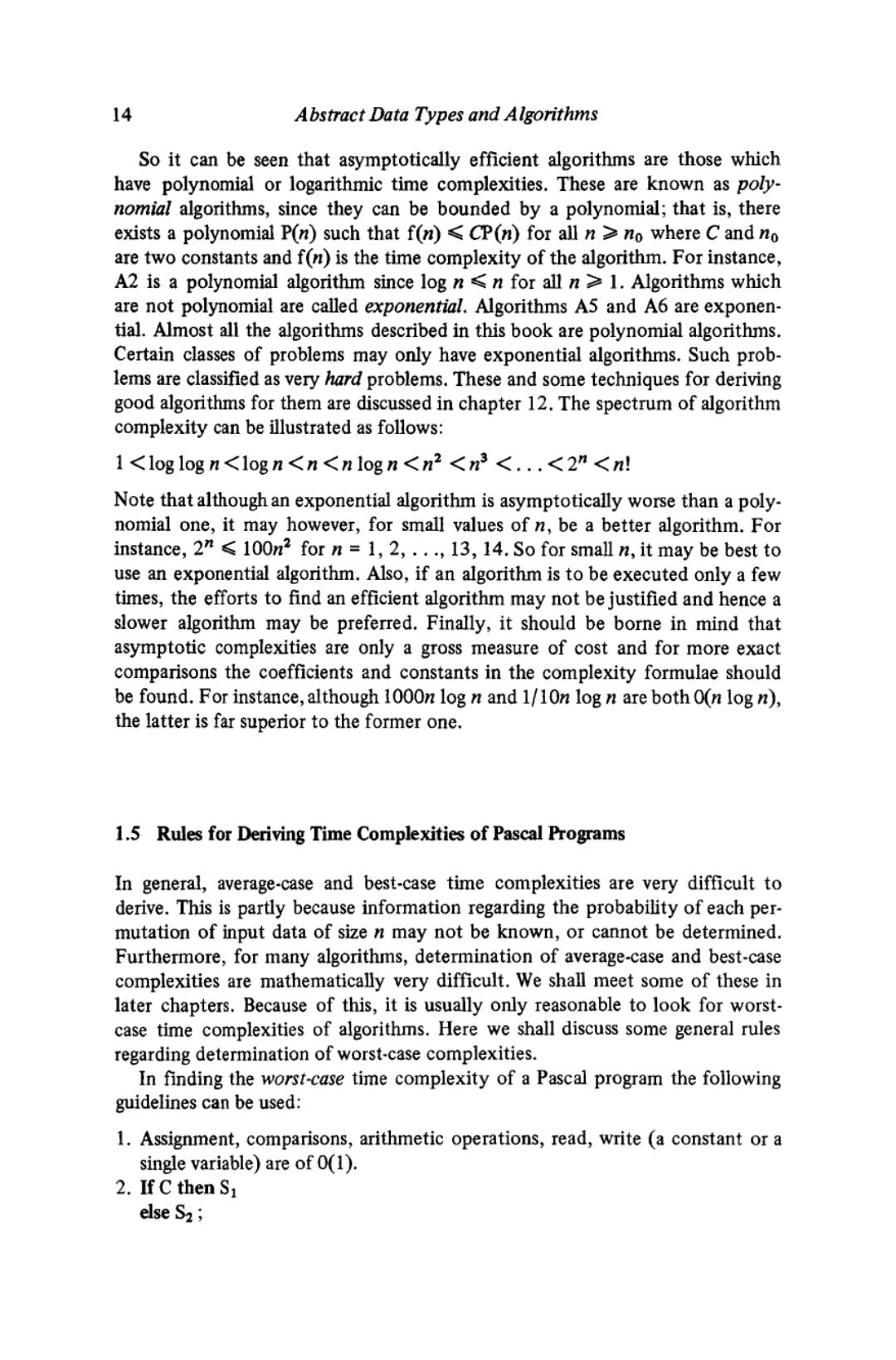
The Complexity of Algorithms 15 needs Te+Max(Ts,,Ts)where Te,Ts and Ts,are time complexities of C,S1 and S2. 3.For loops.The number of times the loop is executed must be multiplied by the time complexity of the body of the loop. 4.while C do S;and repeat S until C; For both these loop constructs we should find the number of times the loop will be executed and multiply this by the complexities of C and S.For instance,the loop of b_search function is executed log2n times.Thus,its time complexity is log2n(0(1))=0(log2n).This simple analysis may not work for all loops.In these cases other properties of the program should be used to infer the time com- plexity.As an example,let us look at the following hypothetical program fragment: size :m; i1=1; while i<n do begin i:=i+1; statement.................o(n) if size 0 then begin Choose a number in the range 1..size and assign it to s; size i=size s; for j=1 to s do statement..........0(n) end end; The while loop above will be executed n-1 times.This is because i is initialised to 1 and is incremented by 1 each time the body of the while loop is executed. Thus statement:will be executed n-1 times.We cannot find the number of times the for loop (inside the while loop)will be executed as a function of i. However,if s is the value of s inside the while loop for a given value of i,then the total number of times statement will be executed iss.The sum of the s values will bes=m,since size is initially set to m and in each iteration of the while loop s is subtracted from size.Thus the total time due to statement2 will be m x 0(n).The total time due to statementi is n x O(n).The time complexity of the entire while loop is n×0(m)+mx0(n)+ 0(1) =0(n2+mn) statement statement2 tests,assignments etc. We shall see examples of such loops in the rest of the book (for instance,see Dijkstra's algorithm of chapter 7)
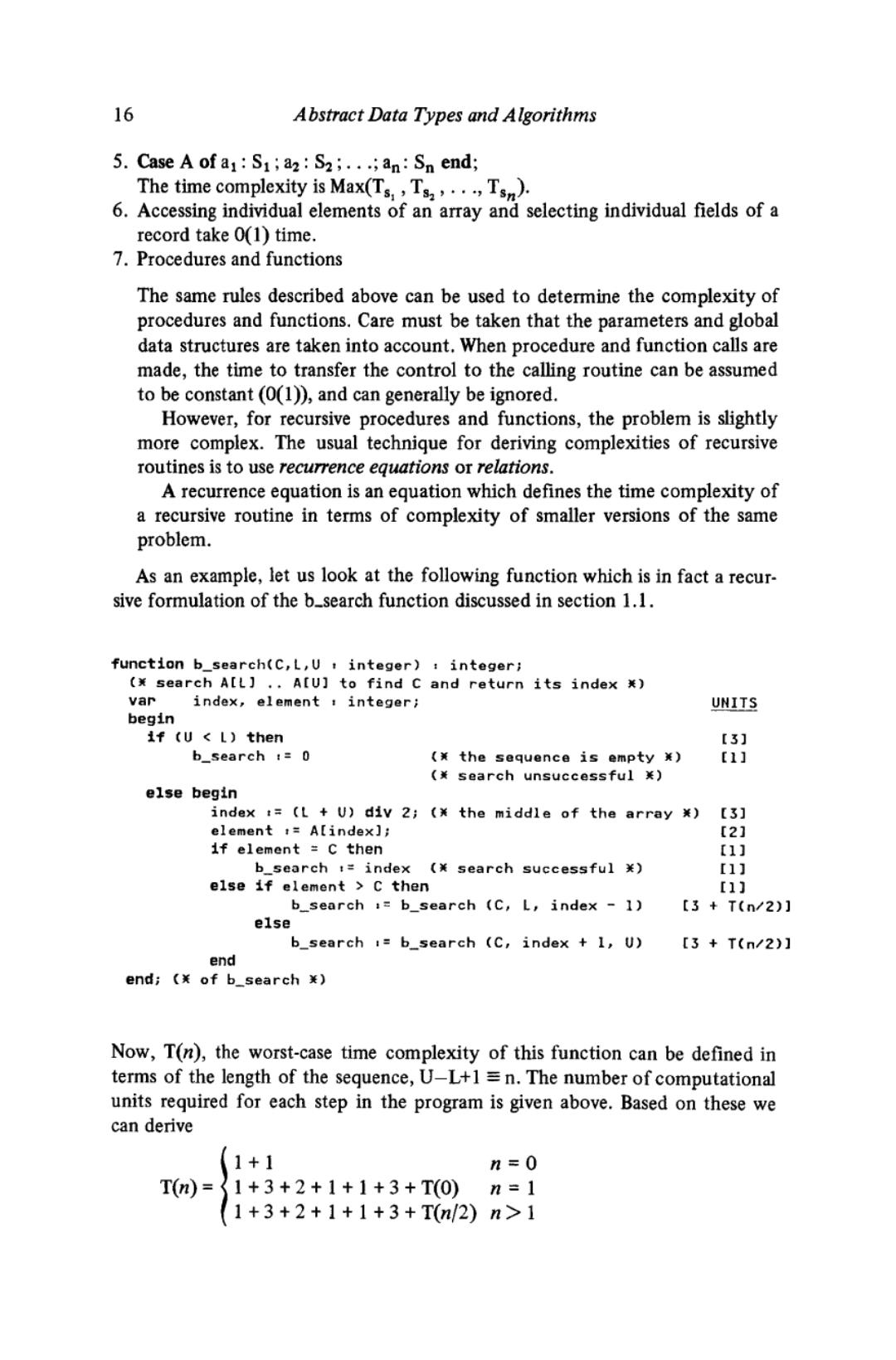
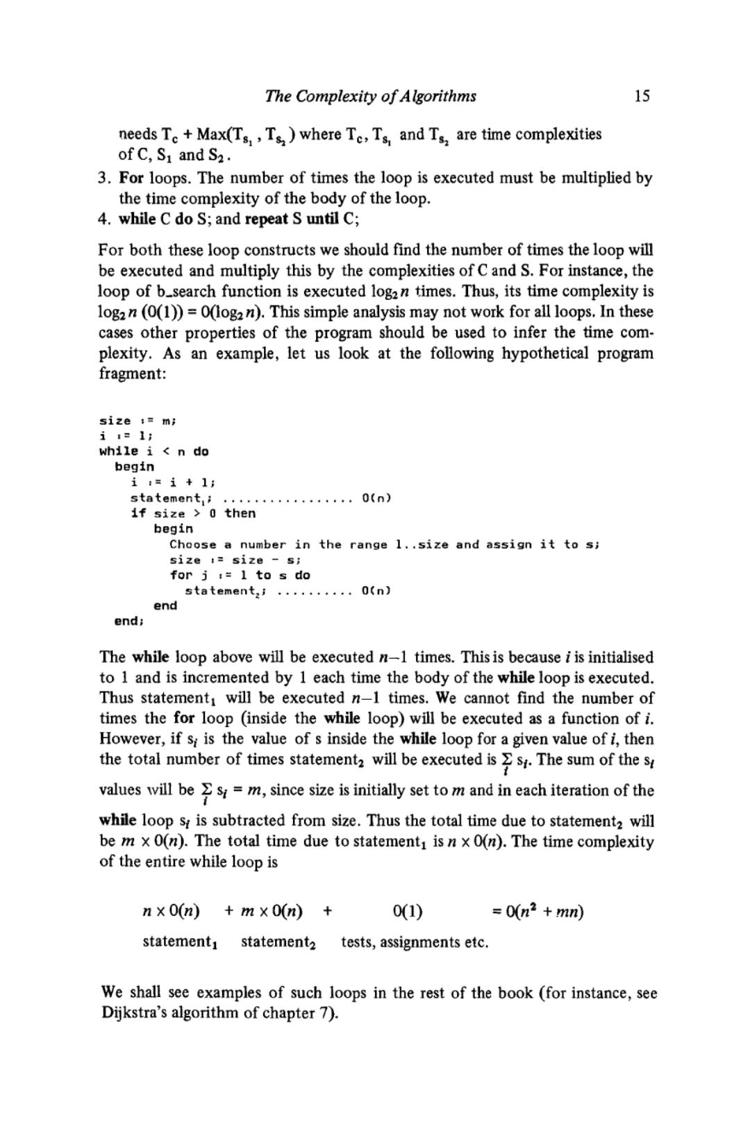
16 Abstract Data Types and Algorithms 5.Case A of a:S1 a2 S2;...;an:Sn end; The time complexity is Max(Ts,T,Ts). 6.Accessing individual elements of an array and selecting individual fields of a record take 0(1)time. 7.Procedures and functions The same rules described above can be used to determine the complexity of procedures and functions.Care must be taken that the parameters and global data structures are taken into account.When procedure and function calls are made,the time to transfer the control to the calling routine can be assumed to be constant (0(1)),and can generally be ignored. However,for recursive procedures and functions,the problem is slightly more complex.The usual technique for deriving complexities of recursive routines is to use recurrence equations or relations. A recurrence equation is an equation which defines the time complexity of a recursive routine in terms of complexity of smaller versions of the same problem. As an example,let us look at the following function which is in fact a recur- sive formulation of the b_search function discussed in section 1.1. function bsearch(C,L,U integer):integer; (x search A[L]..A[U]to find c and return its index x) var index,element integer; UNITS begin if (U L)then 【3] b_search :0 (x the sequence is empty x) [1] (¥search unsuccessful关) else begin index :=(L U)div 2;(x the middle of the array [3] element t=A[index]; [2] if element c then [1] bsearch t=index(¥search successful关) [1] else if element c then [1] b_search b_search (C,L,index 1) [3+T(n/2)J else b_search =b_search (C,index 1,U) 【3+T(n/2)] end end;(¥ofb_search¥) Now,T(n),the worst-case time complexity of this function can be defined in terms of the length of the sequence,U-L+1=n.The number of computational units required for each step in the program is given above.Based on these we can derive 1+1 n=0 T(n)= 1+3+2+1+1+3+T(0)n=1 1+3+2+1+1+3+T(n/2)n>1