
Returns to Buying Winners and Selling Losers 69 returns file.4 All stocks with available returns data in the J months preced- ing the portfolio formation date are included in the sample from which the buy and sell portfolios are constructed. Table I reports the average returns of the different buy and sell portfolios as well as the zero-cost,winners minus losers portfolio,for the 32 strategies described above.The returns of all the zero-cost portfolios (i.e.,the returns per dollar long in this portfolio)are positive.All these returns are statisti- cally significant except for the 3-month/3-month strategy that does not skip a week.Many of the individual t-statistics are sufficiently large to be significant even after considering the fact that we have conducted 32 sepa- rate tests.The probability of obtaining a single t-statistic as large as 4.28 (obtained with the 12-month/3-month strategy that skips a week)with 32 observations is less than 0.0006,as given by the Bonferroni inequality.5 The most successful zero-cost strategy selects stocks based on their returns over the previous 12 months and then holds the portfolio for 3 months.This strategy yields 1.31%per month(shown in Panel A)when there is no time lag between the portfolio formation period and the holding period and it yields 1.49%per month (shown in Panel B)when there is a 1-week lag between the formation period and the holding period.6 The 6-month forma- tion period produces returns of about 1%per month regardless of the holding period.These holding period returns are slightly higher when there is a 1-week lag between the formation period and the holding period (Panel B) than when the formation and holding periods are contiguous(Panel A). Having established that the relative strength strategies are on average quite profitable,we now examine one specific strategy in detail,the 6- month/6-month strategy that does not skip a week between the portfolio formation period and the holding period.The results for this strategy are representative of the results for the other strategies. III.Sources of Relative Strength Profits This section presents two simple return-generating models that allow us to decompose the excess returns documented in the last section and identify the important sources of relative strength profits.The first model allows for factor-mimicking portfolio returns to be serially correlated but requires indi- 4The latest version of the CRSP daily returns file at the time this study was initiated covers the July 1962 to December 1989 period.Monthly returns were obtained by compounding the daily returns recorded in this data set.Since the 12-month/12-month strategy considered here requires lagged returns data over 23 months the first full'calendar year for which we could examine portfolio returns is 1965. The Bonferroni inequality provides a bound for the probability of observing a t-statistic of a certain magnitude with N tests that are not necessarily independent. De Bondt and Thaler (1985)report 1-year holding period returns in their tables that are consistent with our findings here.However,they do not examine strategies based on 1-year horizons in any detail and based on their analysis of longer horizon strategies conclude that the market overreacts
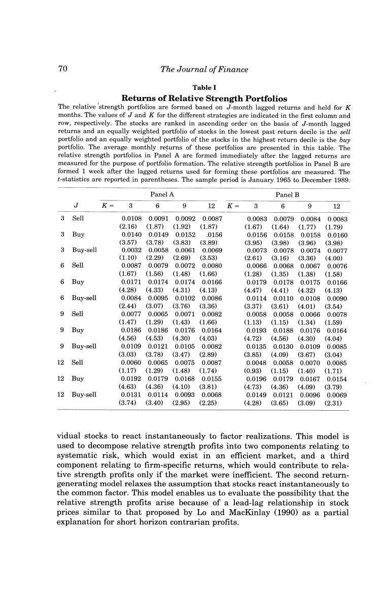
70 The Journal of Finance Table I Returns of Relative Strength Portfolios The relative 'strength portfolios are formed based on J-month lagged returns and held for K months.The values of J and K for the different strategies are indicated in the first column and row,respectively.The stocks are ranked in ascending order on the basis of J-month lagged returns and an equally weighted portfolio of stocks in the lowest past return decile is the sell portfolio and an equally weighted portfolio of the stocks in the highest return decile is the buy portfolio.The average monthly returns of these portfolios are presented in this table.The relative strength portfolios in Panel A are formed immediately after the lagged returns are measured for the purpose of portfolio formation.The relative strength portfolios in Panel B are formed 1 week after the lagged returns used for forming these portfolios are measured.The t-statistics are reported in parentheses.The sample period is January 1965 to December 1989. Panel A Panel B J K= 6 9 12 K- 6 9 12 3 Sell 0.01080.00910.00920.0087 0.00830.00790.0084 0.0083 (2.16) (1.87)(1.92) (1.87) (1.67) (1.64) (1.77) (1.79) 3 Buy 0.01400.01490.0152 .0156 0.0156 0.01580.0158 0.0160 (3.57) (3.78) (3.83) (3.89) (3.95) (3.98) (3.96) (3.98) 3 Buy-sell 0.00320.0058 0.00610.0069 0.00730.00780.00740.0077 (1.10) (2.29) (2.69) (3.53) (2.61) (3.16) (3.36) (4.00) 6 Sell 0.00870.00790.0072 0.0080 0.00660.00680.0067 0.0076 (1.67) (1.56)(1.48) (1.66) (1.28) (1.35) (1.38) (1.58) 6 Buy 0.01710.0174 0.0174 0.0166 0.01790.0178 0.0175 0.0166 (4.28) (4.33) (4.31) (4.13) (4.47) (4.41)(4.32) (4.13) 6 Buy-sell 0.00840.00950.01020.0086 0.01140.01100.0108 0.0090 (2.44) (3.07) (3.76) (3.36) (3.37) (3.61) (4.01) (3.54) 9 Sell 0.00770.0065 0.0071 0.0082 0.00580.0058 0.0066 0.0078 (1.47) (1.29) (1.43) (1.66) (1.13) (1.15)(1.34) (1.59) 9 Buy 0.01860.01860.0176 0.0164 0.01930.0188 0.01760.0164 (4.56) (4.53) (4.30) (4.03) (4.72) (4.56) (4.30) (4.04) 9 Buy-sell 0.0109 0.0121 0.0105 0.0082 0.0135 0.0130 0.0109 0.0085 (3.03) (3.78) (3.47) (2.89) (3.85) (4.09) (3.67) (3.04) 12 Sell 0.00600.00650.00750.0087 0.00480.00580.00700.0085 (1.17) (1.29) (1.48) (1.74) (0.93) (1.15) (1.40) (1.71) 12 Buy 0.01920.0179 0.01680.0155 0.01960.01790.0167 0.0154 (4.63)(4.36) (4.10) (3.81) (4.73) (4.36) (4.09) (3.79) 12 Buy-sell 0.01310.01140.00930.0068 0.01490.01210.0096 0.0069 (3.74) (3.40) (2.95) (2.25) (4.28) (3.65) (3.09) (2.31) vidual stocks to react instantaneously to factor realizations.This model is used to decompose relative strength profits into two components relating to systematic risk,which would exist in an efficient market,and a third component relating to firm-specific returns,which would contribute to rela- tive strength profits only if the market were inefficient.The second return- generating model relaxes the assumption that stocks react instantaneously to the common factor.This model enables us to evaluate the possibility that the relative strength profits arise because of a lead-lag relationship in stock prices similar to that proposed by Lo and MacKinlay (1990)as a partial explanation for short horizon contrarian profits
Returns to Buying Winners and Selling Losers 71 A.A Simple One-Factor Model Consider the following one-factor model describing stock returns: rit ui+bift+eu, E(f)=0 E(e)-0 (1) Cov(eit,f:)=0, i Cov(eit,eit-1)=0, i卡j where u is the unconditional expected return on security i,ri is the return on security i,f is the unconditional unexpected return on a factor- mimicking portfolio,ei:is the firm-specific component of return at time t,and 6,is the factor sensitivity of security i.For the 6-month/6-month strategy that we consider in the rest of this paper the length of a period is 6 months. The superior performance of the relative strength strategies documented in the last section implies that stocks that generate higher than average returns in one period also generate higher than average returns in the period that follows.In other words,these results imply that: E(r:-.lr4-1-7-1>0)>0 and E(rt-Trt-1-7-1<0)<0, where a bar above a variable denotes its cross-sectional average. Therefore, E(r-7)(r4-1-万:-1)}>0. (2) The above cross-sectional covariance equals the expected profits from the zero-cost contrarian trading strategy examined by Lehmann(1990)and Lo and MacKinlay(1990)that weights stocks by their past returns less the past equally weighted index returns.This weighted relative strength strategy (WRSS)is closely related to our strategy.The WRSS yields a profit of 4.5% per dollar long semiannually(t-statistic =2.99)and the correlation between the returns of this strategy and that of the trading strategy examined in the last section is 0.95.The equally weighted decile portfolios are used in most of our empirical tests since they provide relatively more information than the WRSS.However,as the following analysis demonstrates,the closely related WRSS provides a tractable framework for analytically examining the sources of relative strength profits and evaluating the relative importance of each of these sources. 'Our analysis in this subsection is similar to that in Jegadeesh(1987)and Lo and MacKinlay (1990)
72 The Journal of Finance Given the one-factor model defined in (1),the WRSS profits given in expression(2)can be decomposed into the following three terms: E((rit -F)(rit-1-F:-1)}=g2+oCov(f,f:-1) Covi(eit,eit-1), (3) where o2 and are the cross-sectional variances of expected returns and factor sensitivities respectively. The above decomposition suggests three potential sources of the relative strength profits.The first term in this expression is the cross-sectional dispersion in expected returns.Intuitively,since realized returns contain a component related to expected returns,securities that experience relatively high returns in one period can be expected to have higher than average returns in the following period.The second term is related to the potential to time the factor.If the factor portfolio returns exhibit positive serial correla- tion,the relative strength strategy will tend to pick stocks with high b's when the conditional expectation of the factor portfolio return is high.As the above expression demonstrates,the extent to which relative strength strate- gies generate profits because of the serial correlation of the factor portfolio return is a function of the cross-sectional variance of the b's.The last term in the above expression is the average serial covariance of the idiosyncratic components of security returns. To assess whether the existence of relative strength profits imply market inefficiency,it is important to identify the sources of the profits.If the profits are due to either the first or the second term in expression(3)they may be attributed to compensation for bearing systematic risk and need not be an indication of market inefficiency.However,if the superior performance of the relative strength strategies is due to the third term,then the results would suggest market inefficiency. B.The Average Size and Beta of Relative Strength Portfolios This subsection considers the possibility that relative strength strategies systematically pick high-risk stocks and benefit from the first term in expres- sion (3).Table II reports estimates of the two most common indicators of systematic risk,the post-ranking betas of the ten 6-month/6-month relative strength portfolios and the average capitalizations of the stocks in these portfolios.The betas of the extreme past returns portfolios are higher than the average beta for the full sample.In addition,since the beta of the portfolio of past losers is higher than the beta of the portfolio of past winners, the beta of the zero-cost winners minus losers portfolio is negative.The average capitalizations of the stocks in the different portfolios show that the highest and the lowest past returns portfolios consist of smaller than average stocks,with the stocks in the losers portfolios being smaller than the stocks in the winners portfolio.This evidence suggests that the observed relative strength profits are not due to the first source of profits in expression (3)
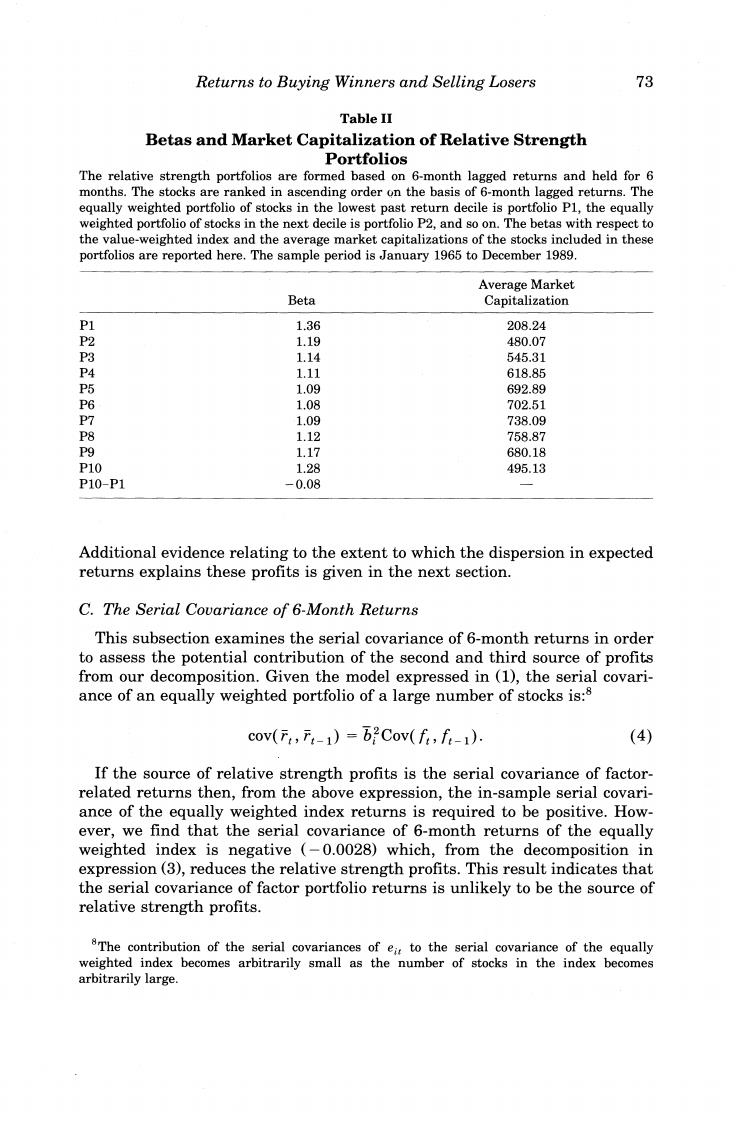
Returns to Buying Winners and Selling Losers 73 Table II Betas and Market Capitalization of Relative Strength Portfolios The relative strength portfolios are formed based on 6-month lagged returns and held for 6 months.The stocks are ranked in ascending order on the basis of 6-month lagged returns.The equally weighted portfolio of stocks in the lowest past return decile is portfolio Pl,the equally weighted portfolio of stocks in the next decile is portfolio P2,and so on.The betas with respect to the value-weighted index and the average market capitalizations of the stocks included in these portfolios are reported here.The sample period is January 1965 to December 1989. Average Market Beta Capitalization P1 1.36 208.24 P2 1.19 480.07 P3 1.14 545.31 P4 1.11 618.85 P5 1.09 692.89 P6 1.08 702.51 P7 1.09 738.09 P8 1.12 758.87 P9 1.17 680.18 P10 1.28 495.13 P10-P1 -0.08 Additional evidence relating to the extent to which the dispersion in expected returns explains these profits is given in the next section. C.The Serial Covariance of 6-Month Returns This subsection examines the serial covariance of 6-month returns in order to assess the potential contribution of the second and third source of profits from our decomposition.Given the model expressed in (1),the serial covari- ance of an equally weighted portfolio of a large number of stocks is:8 cov(,1)=b2Cov(f,f-1). (4) If the source of relative strength profits is the serial covariance of factor- related returns then,from the above expression,the in-sample serial covari- ance of the equally weighted index returns is required to be positive.How- ever,we find that the serial covariance of 6-month returns of the equally weighted index is negative (-0.0028)which,from the decomposition in expression(3),reduces the relative strength profits.This result indicates that the serial covariance of factor portfolio returns is unlikely to be the source of relative strength profits. 8The contribution of the serial covariances of eit to the serial covariance of the equally weighted index becomes arbitrarily small as the number of stocks in the index becomes arbitrarily large