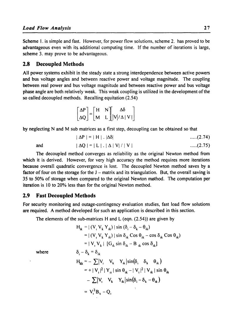
Load Flow Analysis 27 Scheme 1.is simple and fast.However,for power flow solutions,scheme 2.has proved to be advantageous even with its additional computing time.If the number of iterations is large, scheme 3.may prove to be advantageous. 2.8 Decoupled Methods All power systems exhibit in the steady state a strong interdependence between active powers and bus voltage angles and between reactive power and voltage magnitude.The coupling between real power and bus voltage magnitude and between reactive power and bus voltage phase angle are both relatively weak.This weak coupling is utilized in the development of the so called decoupled methods.Recalling equitation(2.54) AP]「HNA8 AQM LJV/AIVI by neglecting N and M sub matrices as a first step,decoupling can be obtained so that |△PI=IH,△δ .(2.74) and I△QI=ILI.I△IVI1IV1 .(2.75) The decoupled method converges as reliability as the original Newton method from which it is derived.However,for very high accuracy the method requires more iterations because overall quadratic convergence is lost.The decoupled Newton method saves by a factor of four on the storage for the J-matrix and its triangulation.But,the overall saving is 35 to 50%of storage when compared to the original Newton method.The computation per iteration is 10 to 20%less than for the original Newton method. 2.9 Fast Decoupled Methods For security monitoring and outage-contingency evaluation studies,fast load flow solutions are required.A method developed for such an application is described in this section. The elements of the sub-matrices H and L (egn.(2.54))are given by Hk=|(V,VkYk)Isin(⑥,-⑧k-ek) =|(V,VkYk)lsinδkCos 0k-cosδCos k) =|V,Vk|[Gk sinδk-Bk cosδkJ where δ,-8k=δk Hw=-∑y,V Y sin(6,δkek) =+V,R1YnI sin ek-1V;R2I Vik I sin ek -∑Y,V Yiksin(6:-δk-ek) V2Bi -Q
Load Flow Analysis 27 Scheme I. is simple and fast. However, for power flow solutions, scheme 2. has proved to be advantageous even with its additional computing time. If the number of iterations is large, scheme 3. may prove to be advantageous. 2.8 Decoupled Methods All power systems exhibit in the steady state a strong interdependence between active powers and bus voltage angles and between reactive power and voltage magnitude. The coupling between real power and bus voltage magnitude and between reactive power and bus voltage phase angle are both relatively weak. This weak coupling is utilized in the development of the so called decoupled methods. Recalling equitation (2.54) ~P] [H NI ~o ] ~Q - M L IVI/~IVI by neglecting Nand M sub matrices as a first step, decoupling can be obtained so that I ~p I = I HI· I~ol and I ~Q I = I L I . I ~ I VI ! I V I ..... (2.74) ..... (2.75) The decoupled method converges as reliability as the original Newton method from which it is derived. However, for very high accuracy the method requires more iterations because overall quadratic convergence is lost. The decoupled Newton method saves by a factor of four on the storage for the J - matrix and its tri-angulation. But, the overall saving is 35 to 50% of storage when compared to the original Newton method. The computation per iteration is 10 to 20% less than for the original Newton method. 2.9 Fast Decoupled Methods For security monitoring and outage-contingency evaluation studies, fast load flow solutions are required. A method developed for such an application is described in this section. The elements of the sub-matrices Hand L (eqn. (2.54» are given by H'k = I (VI V k Ylk ) I sin (01 - Ok - elk) where = I (VI V k Ylk ) I sin 0lk Cos elk - cos 0lk Cos elk) = I VI Vk I [Glk sin 0lk - B Ik cos ~\d 01 - Ok = 0lk Hkk = - 2:IVI Vk YI~ Isin(o, Ok elk) = + I VI1 21 YII I sin elk -I Vi 121 Vlk I sin elk - 2:IVI Vk Yiklsin(Oi -Ok -elk)
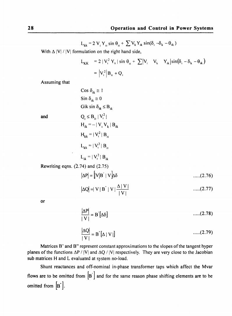
28 Operation and Control in Power Systems Lkk=2V,Y,sin6,+∑VYik sin(6,δk-6k) With AVI/V formulation on the right hand side, LKk=2IV2 YI sin.+∑VVY,ksin6,-δk-ek) =V2B +Q Assuming that Cosδk=1 Sinδk=0 Gik sinδk≤Bk and Q,≤BIV2I Hik=-1V VkIBk Hkk=|V21B。 Lkk =IV21B Lk=IV21Bk Rewriting eqns.(2.74)and(2.75) IAP=VB'IVAδ ..(2.76) VV (2.77) or AP=BA) (2.78) IV A=B"AIVi .(2.79) 1V1 Matrices B'and B"represent constant approximations to the slopes of the tangent hyper planes of the functions AP/V]and AQ/VI respectively.They are very close to the Jacobian sub matrices H and L evaluated at system no-load. Shunt reactances and off-nominal in-phase transformer taps which affect the Mvar flows are to be omitted from B and for the same reason phase shifting elements are to be omited fromB
28 Operation and Control in Power Systems Lkk = 2 V, Y" sin ell + 2: Vk Y,k sin(o, -()k - e,k) With lllVI / IVI formulation on the right hand side, LKK = 2 I V,2 YII I sin ell + 2: lv, Vk Y,k Isin{o, - Ok - e,k) Assuming that and Cos O,k == I Sin O,k == 0 Gik sin 0ik ~ B,k 0, ~ Bi , IV?I Hik = -I V, V k I B,k Hkk = I V,2 1 B" Lkk = I V,21 B" L,k = I V,2 1 B,k Rewriting eqns. (2.74) and (2.75) or III pi = ~VIB' I V ~O IllOI =1 V I B" I V III I V I IVI III pi = B'[~o] IVI IllOI = B"[~ I V I] IVI ..... (2.76) ..... (2.77) ..... (2.78) ..... (2.79) Matrices B' and B" represent constant approximations to the slopes of the tangent hyper planes of the functions ~p / IVI and 110 / IVI respectively. They are very close to the Jacobian sub matrices Hand L evaluated at system no-load. Shunt reactances and off-nominal in-phase transformer taps which affect the Mvar flows are to be omitted from [B'] and for the same reason phase shifting elements are to be omitted from [B"]
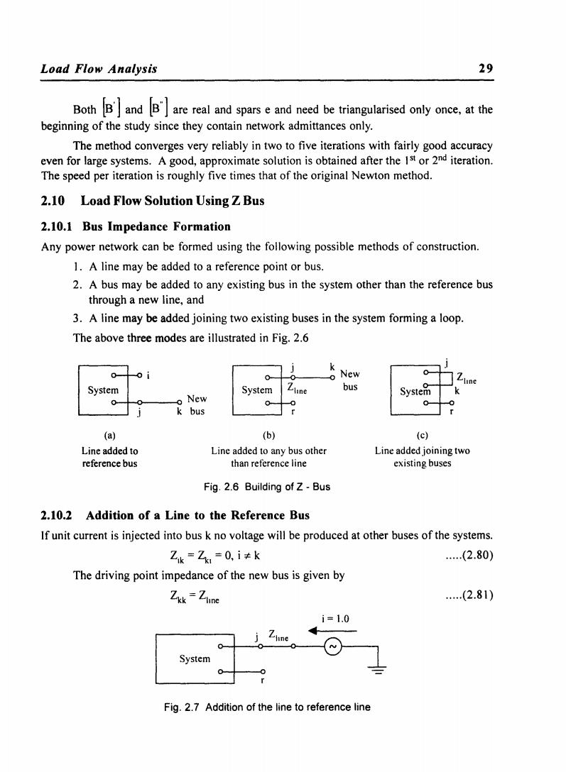
Load Flow Analysis 29 BothBand Bare real and sparseand need be triangularised only once.at the beginning of the study since they contain network admittances only. The method converges very reliably in two to five iterations with fairly good accuracy even for large systems.A good,approximate solution is obtained after the Ist or 2nd iteration. The speed per iteration is roughly five times that of the original Newton method. 2.10 Load Flow Solution Using Z Bus 2.10.1 Bus Impedance Formation Any power network can be formed using the following possible methods of construction. 1.A line may be added to a reference point or bus. 2.A bus may be added to any existing bus in the system other than the reference bus through a new line,and 3.A line may be added joining two existing buses in the system forming a loop. The above three modes are illustrated in Fig.2.6 0 New System System bus System 0 o New 0 k bus (a) (b) (c) Line added to Line added to any bus other Line added joining two reference bus than reference line existing buses Fig.2.6 Building of Z-Bus 2.10.2 Addition of a Line to the Reference Bus If unit current is injected into bus k no voltage will be produced at other buses of the systems. Zk=Zk,=0,i≠k .(2.80) The driving point impedance of the new bus is given by Zkk=Zlne ..(2.81) i=1.0 System Fig.2.7 Addition of the line to reference line
Load Flow Analysis 29 Both ~.] and [B"] are real and spars e and need be triangularised only once, at the beginning of the study since they contain network admittances only. The method converges very reliably in two to five iterations with fairly good accuracy even for large systems. A good, approximate solution is obtained after the pI or 2nd iteration. The speed per iteration is roughly five times that of the original Newton method. 2.10 Load Flow Solution Using Z Bus 2.10.1 Bus Impedance Formation Any power network can be formed using the following possible methods of construction. I. A line may be added to a reference point or bus. 2. A bus may be added to any existing bus in the system other than the reference bus through a new line, and 3. A line may be added joining two existing buses in the system forming a loop. The above three modes are illustrated in Fig. 2.6 S,,,,~_i __ O New ~ k bus (a) Line added to reference bus k 0-+-<>----0 New System lime (b) Line added to any bus other than reference line bus Fig. 2.6 Building of Z - Bus 2.10.2 Addition of a Line to the Reference Bus lime Bi System r k (c) Line added joining two existing buses If unit current is injected into bus k no voltage will be produced at other buses of the systems. Zlk = ~I = 0, i '* k ..... (2.80) The driving point impedance of the new bus is given by ..... (2.81 ) i = 1.0 . l ... ~I---- System :-+-----<1 J ~ l Fig. 2.7 Addition of the line to reference line
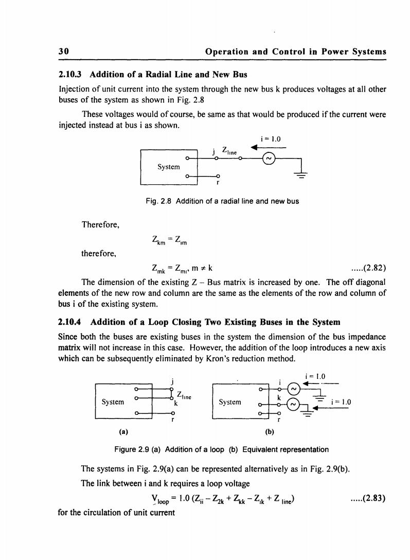
30 Operation and Control in Power Systems 2.10.3 Addition of a Radial Line and New Bus Injection of unit current into the system through the new bus k produces voltages at all other buses of the system as shown in Fig.2.8 These voltages would of course,be same as that would be produced if the current were injected instead at bus i as shown. i=1.0 System Fig.2.8 Addition of a radial line and new bus Therefore, Zkm=Zim therefore, Zmk=Zm,m≠k .(2.82) The dimension of the existing Z-Bus matrix is increased by one.The off diagonal elements of the new row and column are the same as the elements of the row and column of bus i of the existing system. 2.10.4 Addition of a Loop Closing Two Existing Buses in the System Since both the buses are existing buses in the system the dimension of the bus impedance matrix will not increase in this case.However,the addition of the loop introduces a new axis which can be subsequently eliminated by Kron's reduction method. System =i=1.0 (a) (b) Figure 2.9(a)Addition of a loop (b)Equivalent representation The systems in Fig.2.9(a)can be represented alternatively as in Fig.2.9(b) The link between i and k requires a loop voltage Vloop=1.0 (Zi -Z2k Zkk -Zik +Z lime) .(2.83) for the circulation of unit current
30 Operation and Control in Power Systems 2.10.3 Addition of a Radial Line and New Bus Injection of unit current into the system through the new bus k produces voltages at all other buses of the system as shown in Fig. 2.8 These voltages would of course, be same as that would be produced if the current were injected instead at bus i as shown. i = 1.0 . Z .... ~I---- System :>-+------<I J~ l Fig. 2.8 Addition of a radial line and new bus Therefore, therefore, Zmk = Zml' m -:t:. k ..... (2.82) The dimension of the existing Z - Bus matrix is increased by one. The off diagonal elements of the new row and column are the same as the elements of the row and column of bus i of the existing system. 2.10.4 Addition of a Loop Closing Two Existing Buses in the System Since both the buses are existing buses in the system the dimension of the bus impedance matrix will not increase in this case. However, the addition of the loop introduces a new axis which can be subsequently eliminated by Kron's reduction method. :TikZ,tne System o ___ +--4~ ~ _~o_ IV - 1=1.0 ~ '-------' r System (a) (b) Figure 2.9 (a) Addition of a loop (b) Equivalent representation The systems in Fig. 2.9(a) can be represented alternatively as in Fig. 2.9(b). The link between i and k requires a loop voltage "Yloop = 1.0 (Zii - Z2k + Zkk - Zlk + Z line) for the circulation of unit current ..... (2.83)
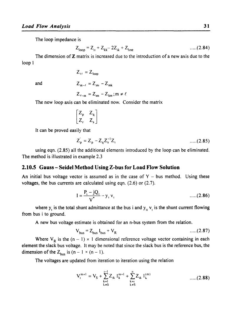
Load Flow Analysis 31 The loop impedance is Zloop=Zu+Zkk-2Zik+Zline .(2.84) The dimension of Z matrix is increased due to the introduction of a new axis due to the loop I Z=Zloop and Zm-t Zm -Zmk Z,-m=Zm-Zkm;m≠C The new loop axis can be eliminated now.Consider the matrix It can be proved easily that Z。=Z。-ZZ,Z ..(2.85) using eqn.(2.85)all the additional elements introduced by the loop can be eliminated. The method is illustrated in example 2.3 2.10.5 Gauss-Seidel Method Using Z-bus for Load Flow Solution An initial bus voltage vector is assumed as in the case of Y-bus method.Using these voltages,the bus currents are calculated using eqn.(2.6)or(2.7). 1=-0-yv, ..(2.86) where y,is the total shunt admittance at the bus i and y v,is the shunt current flowing from bus i to ground. A new bus voltage estimate is obtained for an n-bus system from the relation. Vous=Zous Ibus+VR .(2.87) Where Vg is the(n-1)x I dimensional reference voltage vector containing in each element the slack bus voltage.It may be noted that since the slack bus is the reference bus,the dimension of the Zous is(n-1 x (n-1). The voltages are updated from iteration to iteration using the relation 1= Vm1=V+∑Z+∑2k1m (2.88) k=}
Load Flow Analysis 31 The loop impedance is Zloop = ZII + Zkk - 2ZIk + Zhne ..... (2.84) The dimension of Z matrix is increased due to the introduction of a new axis due to the loop 1 and Zr_m = Zun -Zkm;m 7: e The new loop axis can be eliminated now. Consider the matrix It can be proved easily that ..... (2.85) using eqn. (2.85) all the additional elements introduced by the loop can be eliminated. The method is illustrated in example 2.3 2.10.5 Gauss - Seidel Method Using Z-bus for Load Flow Solution An initial bus voltage vector is assumed as in the case of Y - bus method. Using these voltages, the bus currents are calculated using eqn. (2.6) or (2.7). P .Q 1= I-J I_ y v y' I I ..... (2.86) where YI is the total shunt admittance at the bus i and YII VI is the shunt current flowing from bus i to ground. A new bus voltage estimate is obtained for an n-bus system from the relation. Ybus = Zbus Ibus + YR ..... (2.87) Where Y R is the (n - 1) x 1 dimensional reference voltage vector containing in each element the slack bus voltage. It may be noted that since the slack bus is the reference bus, the dimension of the Zbus is (n - I x (n - I). The voltages are updated from iteration to iteration using the relation ..... (2.88)