232 Computational Mechanics of Composite Materials 2e+007 1e+007 8e+006 6e+006 4e+006 2e+006 042 02站02d1500话00动0防009040045005 Figure 5.2.Expected values of fatigue cycles number (EdN) 5e+006 4e+006+ 3e+006+ 2e+006 1e+006 0.25 0201569100s0i500900io590040046005 Figure 5.3.Standard deviations of fatigue cycles number (odN) Especially interesting here is a comparison between deterministic analysis and expected values obtained for analogous input data.It is seen that the expectations are essentially greater than the deterministic output,which results from(5.17),for instance.The difference increases nonlinearly together with an increase in the coefficient of variation of the stress amplitude Ao.In the case of a(Ao)=25%this difference is equal to about 20%of the relevant deterministic values.This result can be used as the safety factor which could be proposed for deterministic analysis as S=1.2 for an analogous range of random variability of the stress amplitude. Furthermore,it is seen that the final crack length is remarkably more decisive for fatigue cycle number(even in a random case)than the coefficient of variation of the stress amplitude. As shown in Figure 5.3,the variability of the examined standard deviation of Ao is essentially different from that typical for deterministic and expected values. The influences of final crack length and input coefficient of variation are almost
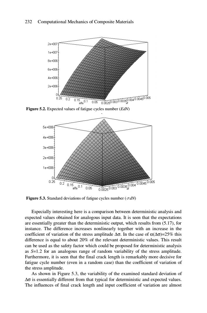
232 Computational Mechanics of Composite Materials Figure 5.2. Expected values of fatigue cycles number (EdN) Figure 5.3. Standard deviations of fatigue cycles number (sdN) Especially interesting here is a comparison between deterministic analysis and expected values obtained for analogous input data. It is seen that the expectations are essentially greater than the deterministic output, which results from (5.17), for instance. The difference increases nonlinearly together with an increase in the coefficient of variation of the stress amplitude ∆σ. In the case of α(∆σ)=25% this difference is equal to about 20% of the relevant deterministic values. This result can be used as the safety factor which could be proposed for deterministic analysis as S=1.2 for an analogous range of random variability of the stress amplitude. Furthermore, it is seen that the final crack length is remarkably more decisive for fatigue cycle number (even in a random case) than the coefficient of variation of the stress amplitude. As shown in Figure 5.3, the variability of the examined standard deviation of ∆σ is essentially different from that typical for deterministic and expected values. The influences of final crack length and input coefficient of variation are almost

Fracture and Fatigue Analysis of Composites 233 the same for 25%increases of both parameters.Considering the above it can be concluded that the influence of the random character in fatigue cycle number is important in higher than first order probabilistic moments computations.It is clear that the presented symbolic computation methodology can be next exploited in the determination of stochastic sensitivity gradients of probabilistic moments of the fatigue cycle number with respect to particular random characteristics of the chosen input variables appearing in the fatigue life cycles formula.In particular,it will enable us to compare the sensitivity of various fatigue models with respect to the same parameters in which the sensitivity gradients are the most reasonable and realistic.The situation would be definitely more complicated if the variation of stress amplitude together with fatigue cycle number is analysed.Random fluctuations of Ao in time should be taken into account in this case and,therefore, Ao(o)=Ao(o,t)is to be considered as a resulting nonstationary random process. 5.3 Computational Issues Since the deterministic equations are valid for the Monte Carlo simulation analysis as well,then the essential theoretical differences are observed in the case of perturbation based analysis.The corresponding fatigue-oriented SFEM model begins with the new description of the material properties,where the stiffness reduction approach can result in the following equations for the Young modulus, Poisson ratio and material density as well as spring stiffness for interface modelling e(n)=eo(1-D(n)),v(n)=vo(1-D(n)) p(n)=p1-D(m),k(n)=k1-D(m) (5.27) Therefore,the first two probabilistic moments for the Young modulus can be represented as Ele(n)]=Eleo](1-ELD(n)]) (5.28) Var(e(n))=Var(eo(1-D(n)))=Var(eo)Var(1-D(n)) (5.29) and up to the second order perturbation equations are rewritten in the incremental formulation as follows: zeroth order MB(m)△8(n)+C(n)△8(m)+K9s(m)△q8(m)=△Q&m) (5.30) first order
Fracture and Fatigue Analysis of Composites 233 the same for 25% increases of both parameters. Considering the above it can be concluded that the influence of the random character in fatigue cycle number is important in higher than first order probabilistic moments computations. It is clear that the presented symbolic computation methodology can be next exploited in the determination of stochastic sensitivity gradients of probabilistic moments of the fatigue cycle number with respect to particular random characteristics of the chosen input variables appearing in the fatigue life cycles formula. In particular, it will enable us to compare the sensitivity of various fatigue models with respect to the same parameters in which the sensitivity gradients are the most reasonable and realistic. The situation would be definitely more complicated if the variation of stress amplitude together with fatigue cycle number is analysed. Random fluctuations of ∆σ in time should be taken into account in this case and, therefore, ∆σ(ω)=∆σ(ω,t) is to be considered as a resulting nonstationary random process. 5.3 Computational Issues Since the deterministic equations are valid for the Monte Carlo simulation analysis as well, then the essential theoretical differences are observed in the case of perturbation based analysis. The corresponding fatigue-oriented SFEM model begins with the new description of the material properties, where the stiffness reduction approach can result in the following equations for the Young modulus, Poisson ratio and material density as well as spring stiffness for interface modelling ( ) ( ) 1 ( ) 0 e n = e − D n , ( ) ( ) 1 ( ) 0 ν n =ν − D n ( ) ( ) 1 ( ) ρ n = ρ0 − D n , ( ) ( ) 1 ( ) k n = k0 − D n (5.27) Therefore, the first two probabilistic moments for the Young modulus can be represented as [ ( )] [ ]( ) 1 [ ( )] E e n = E e0 − E D n (5.28) ( ( )) ( ) () ( ) ( ) 1 ( ) 1 ( ) 0 0 Var e n = Var e − D n = Var e Var − D n (5.29) and up to the second order perturbation equations are rewritten in the incremental formulation as follows: • zeroth order ( ) ( ) ( ) ( ) ( ) ( ) ( ) 0 0 0 0 0 0 0 Mαβ n ∆q&& β n +Cαβ n ∆q&β n + Kαβ n ∆qβ n = ∆Qα n (5.30) • first order
234 Computational Mechanics of Composite Materials Msm)△B(m)+Cm)△站(m)+K8sn)△qi(n)=△Q(m+ (5.31) -MBm)△B(m+Ca3(m)△B(m)+K0m△qBm) second order M8m)△9}m)+C8n)△}(m)+K8n)Aq}m) =AQam-(Mgm)△8m)+CBm)△i8(m)+KBn)△gBm) (5.32) -(Mm)△馆m+Cam)△im)+KB(m)Aqim)} Cov(b"(n).b"(n)) where the stiffness matrix perturbation orders are defined as K品(m=amK品(m)+oK品m)= (5.33) =SC(n)BjaBuBd+JOj(n-1)Pxa.PB.jdQ Ω so the dynamical structural response is given in the form △8=8(n+)-8m) (5.34) The situation is more complicated when the crack phenomenon is considered apart from the material stochasticity and nonlinearity.In such a situation so-called direct methods are used or special purpose enriched finite elements with crack tip modelling can be applied alternatively.In the latter case,the displacements near the crack tip can be defined as (u=Kif.+Kn8. v=Kif +Kngv (5.35) while the near field component f can be rewritten as (5.36) {moe-小o号-m}ne+la号-sn} where o denotes the orientation angle of a crack,which is measured from the positive x axis,r and 0 are polar coordinates with origin at the crack tip and
234 Computational Mechanics of Composite Materials ( ) ( ) ( ) ( ) ( ) ( ) ( ) ( ) ( ) ( ) ( ) ( ) ( ) ( ) , 0 , 0 , 0 0 , 0 , 0 , , M n q n C n q n K n q n M n q n C n q n K n q n Q n r r r r r r r αβ β αβ β αβ β αβ β αβ β αβ β α − ∆ + ∆ + ∆ ∆ + ∆ + ∆ = ∆ + && & && & (5.31) • second order { ( ) ( )} ( ) ( ), ( ) ( ) ( ) ( ) ( ) ( ) ( ) ( ) ( ) ( ) ( ) ( ) ( ) ( ) ( ) ( ) ( ) ( ) ( ) ( ) , , , , , , , , 0 , 0 , 0 0 (2) 0 (2) 0 (2) Cov b n b n M n q n C n q n K n q n Q n M n q n C n q n K n q n M n q n C n q n K n q n r s r s r s r s rs rs rs rs αβ β αβ β αβ β α αβ β αβ β αβ β αβ β αβ β αβ β − ∆ + ∆ + ∆ = ∆ − ∆ + ∆ + ∆ ∆ + ∆ + ∆ && & && & && & (5.32) where the stiffness matrix perturbation orders are defined as ∫ ∫ Ω Ω = Ω + − Ω = + = C n B B d n d K n K n K n ijkl ij kl ij k i k j con , , (.) (.) ( ) (.) ( ) (.) ( ) ( 1) ( ) ( ) ( ) α β α β αβ σ αβ αβ σ ϕ ϕ (5.33) so the dynamical structural response is given in the form ( 1) ( ) (.) (.) (.) q q n q n β β β ∆&& = && + − && (5.34) The situation is more complicated when the crack phenomenon is considered apart from the material stochasticity and nonlinearity. In such a situation so-called direct methods are used or special purpose enriched finite elements with crack tip modelling can be applied alternatively. In the latter case, the displacements near the crack tip can be defined as ⎩ ⎨ ⎧ = + = + I v II v I u II u v K f K g u K f K g (5.35) while the near field component fu can be rewritten as ( ) ( ) ⎭ ⎬ ⎫ ⎥ ⎦ ⎤ ⎢ ⎣ ⎡ + − ⎩ ⎨ ⎧ −⎥ ⎦ ⎤ ⎢ ⎣ ⎡ − − = 2 3 sin 2 sin 2 1 sin 2 3 cos 2 cos 2 1 cos 4 2 1 θ θ φ γ θ θ φ γ π r G fu (5.36) where φ denotes the orientation angle of a crack, which is measured from the positive x axis, r and θ are polar coordinates with origin at the crack tip and
Fracture and Fatigue Analysis of Composites 235 measured from the crack angle,G is shear modulus,while y denotes y=3-4v for plane strain problems or isq tv for the plane stress analyses.The 1+v corresponding SFEM equations for displacements near the crack tip are rewritten using(5.36),while the stress intensity factors are computed using BEM or FEM techniques or,alternatively,are derived mathematically starting from stress equilibrium and displacement compatibility equations.The numerical results of SFEM analysis for composites with and/or without interface and volumetric microdefects are presented in [193,194],while in the case of the cracked medium they can be found in [33]. Alternatively,the structural microdefects are modelled by spherical voids during the ductile type fatigue fracture.Let us assume that the total number of the microdefects is equal to Ma,their radius is denoted by Ra in the composite component indexed with a.Adopting further that both of them are functions of the fatigue cycle,the modified elasticity tensor components can be calculated using stiffness reduction of the Young modulus and Poisson ratio as follows: C(n)=1- rM a(n)Ra(n) ,(n) 1 πM.(nRn) v.(n) 2。 Ma(n)R2(n) (5.37) 6tδ+duδt) πM.(n)R2(n) (n) The use of more advanced deterministic theories is known from the literature. However equivalent stochastic models are not available now.Similarly to a solid model with deterministic and stochastic microvoids,the stiffness reduction approach for cracked media can be applied as well [267].The following material data are adopted for n=0:Young modulus Em=2.1 E11,Poisson ratio vi=0.3, expected value of microvoids radius E[r]=0.1 and standard deviation of microvoids radius o(r)=0.01,expected value of microvoids total number E[M]=1 and variance of microvoids total number Var(M)=0.The Young modulus is taken with +10% deviations from the mean value the microvoid ratio variability is included in the interval [1.0].Therefore an adequate visualisation of the component Ccan be obtained,cf.Figure 5.4
Fracture and Fatigue Analysis of Composites 235 measured from the crack angle, G is shear modulus, while γ denotes γ = 3 − 4ν for plane strain problems or is equal to ν ν γ + − = 1 3 for the plane stress analyses. The corresponding SFEM equations for displacements near the crack tip are rewritten using (5.36), while the stress intensity factors are computed using BEM or FEM techniques or, alternatively, are derived mathematically starting from stress equilibrium and displacement compatibility equations. The numerical results of SFEM analysis for composites with and/or without interface and volumetric microdefects are presented in [193,194], while in the case of the cracked medium they can be found in [33]. Alternatively, the structural microdefects are modelled by spherical voids during the ductile type fatigue fracture. Let us assume that the total number of the microdefects is equal to Ma, their radius is denoted by Ra in the composite component indexed with a. Adopting further that both of them are functions of the fatigue cycle, the modified elasticity tensor components can be calculated using stiffness reduction of the Young modulus and Poisson ratio as follows: ( ) ⎪ ⎪ ⎪ ⎭ ⎪ ⎪ ⎪ ⎬ ⎫ ⎟ ⎟ ⎠ ⎞ ⎜ ⎜ ⎝ ⎛ ⎟ ⎟ ⎠ ⎞ ⎜ ⎜ ⎝ ⎛ Ω + − + × + ⎪ ⎪ ⎪ ⎩ ⎪ ⎪ ⎪ ⎨ ⎧ ⎟ ⎟ ⎠ ⎞ ⎜ ⎜ ⎝ ⎛ ⎟ ⎟ ⎠ ⎞ ⎜ ⎜ ⎝ ⎛ Ω − − ⎟ ⎟ ⎠ ⎞ ⎜ ⎜ ⎝ ⎛ ⎟ ⎟ ⎠ ⎞ ⎜ ⎜ ⎝ ⎛ Ω + − ⎟ ⎟ ⎠ ⎞ ⎜ ⎜ ⎝ ⎛ Ω − × ⎟ ⎟ ⎠ ⎞ ⎜ ⎜ ⎝ ⎛ Ω = − ( ) ( ) ( ) 2 1 1 ( ) ( ) ( ) ( ) 1 2 1 ( ) ( ) 1 1 ( ) ( ) ( ) 1 ( ) ( ) ( ) ( ) 1 2 2 2 2 2 ( ) ( ) n M n R n n M n R n n M n R n n M n R n E n M n R n C n a a a a ik jl il jk ij kl a a a a a a a a a a a a a a eff a a ijkl a ν π δ δ δ δ δ δ ν π ν π ν π π (5.37) The use of more advanced deterministic theories is known from the literature. However equivalent stochastic models are not available now. Similarly to a solid model with deterministic and stochastic microvoids, the stiffness reduction approach for cracked media can be applied as well [267]. The following material data are adopted for n=0: Young modulus Em=2.1 E11, Poisson ratio νm=0.3, expected value of microvoids radius E[r]=0.1 and standard deviation of microvoids radius σ(r)=0.01, expected value of microvoids total number E[M]=1 and variance of microvoids total number Var(M)=0. The Young modulus is taken with ±10% deviations from the mean value the microvoid ratio variability is included in the interval [0,1.0]. Therefore an adequate visualisation of the component ( ) 1111 eff C can be obtained, cf. Figure 5.4

236 Computational Mechanics of Composite Materials 4.8e+011 4.6e+011 4.4e011手 4.2e0113 4e+011 3.8e+011 3.6e+0113 3.4e+011 3.2e+011 1.9e+011 0 2e+011 02 2.1e+011 0.4 0.6r 2.2e+011 0.8 2.3e+0111 Figure 5.4.Parameter variability of C for damaged homogeneous solid Analysing the effective tensor surface,the expected linear dependence of this tensor on the Young modulus is observed as well as the nonlinear dependence on the microvoid mean radius (greater sensitivity to geometrical parameters of the structural defects).If only the statistical information about the input parameters is available,then the elasticity tensor can be rewritten using its first two probabilistic moments and introduced directly in SFEM analysis.If stochastic analysis in the elastoplastic range is necessary,the corresponding extension of the models presented in [355]can be applied.The microvoid volumetric ratio parameter is to be replaced with the two-parameter approach shown above and the probabilistic moments of these parameters are to be inserted as a function of the fatigue cycle. As was mentioned before,the main goal of the homogenisation procedure is to find effective material properties of the homogeneous material,equivalent to the original composite.The most simplified method is to use the spatial average as the homogenised property and it is still used in terms of effective mass density,which can be rewritten for the nth cycle of fatigue analysis as pea(m)=(pn)a (5.38) Analogous homogenisation rule is applied in the case of heat capacity in transient heat transfer analysis and related thermoelastic or thermoelastoplastic coupled analyses of composites.The homogenisation of the elasticity tensor components is definitely more complicated and is usually carried out as C'm)=(C0m)。+o,um》。,forijk1l,2,3 (5.39) where (n)are the homogenisation function depending on the fatigue cycle
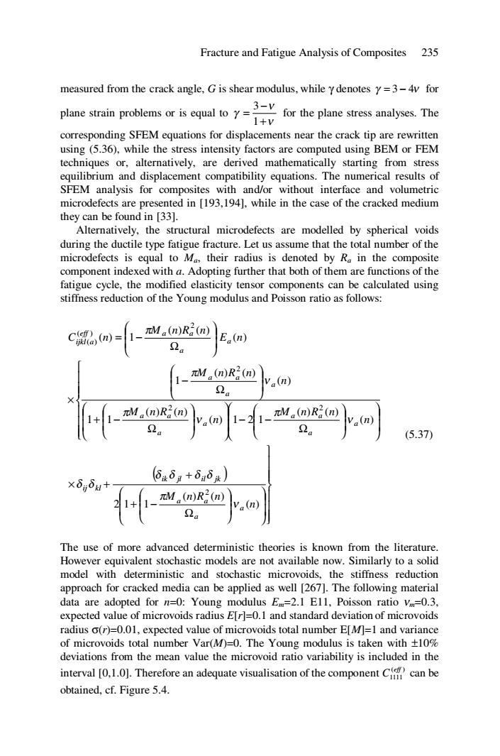
236 Computational Mechanics of Composite Materials Figure 5.4. Parameter variability of ( ) 1111 eff C for damaged homogeneous solid Analysing the effective tensor surface, the expected linear dependence of this tensor on the Young modulus is observed as well as the nonlinear dependence on the microvoid mean radius (greater sensitivity to geometrical parameters of the structural defects). If only the statistical information about the input parameters is available, then the elasticity tensor can be rewritten using its first two probabilistic moments and introduced directly in SFEM analysis. If stochastic analysis in the elastoplastic range is necessary, the corresponding extension of the models presented in [355] can be applied. The microvoid volumetric ratio parameter is to be replaced with the two-parameter approach shown above and the probabilistic moments of these parameters are to be inserted as a function of the fatigue cycle. As was mentioned before, the main goal of the homogenisation procedure is to find effective material properties of the homogeneous material, equivalent to the original composite. The most simplified method is to use the spatial average as the homogenised property and it is still used in terms of effective mass density, which can be rewritten for the nth cycle of fatigue analysis as Ω ( ) = ( ) ( ) n n eff ρ ρ (5.38) Analogous homogenisation rule is applied in the case of heat capacity in transient heat transfer analysis and related thermoelastic or thermoelastoplastic coupled analyses of composites. The homogenisation of the elasticity tensor components is definitely more complicated and is usually carried out as ( ) Ω Ω ( ) = ( ) + ( ) ( ) ( ) C n C n ij kl n a ijkl eff ijkl σ χ , for i,j,k,l=1,2,3 (5.39) where ) (n χ kl are the homogenisation function depending on the fatigue cycle