40 Computational Mechanics of Composite Materials b0 X 2 Figure 2.4.Bubble interface defects in the fibre-reinforced composite △2c R R -△2c Figure 2.5.Interphase for bubble interface defects As can be easily seen in the above relation,there holds Sa=π+la+3arl-R2l (2.31) In a similar way the variance is derived as wob.w (2.32)
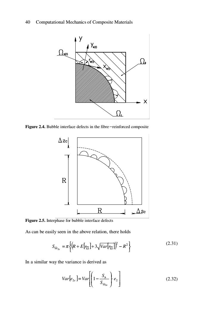
40 Computational Mechanics of Composite Materials Figure 2.4. Bubble interface defects in the fibre-reinforced composite Figure 2.5. Interphase for bubble interface defects As can be easily seen in the above relation, there holds ( ) [ ] [ ] ⎭ ⎬ ⎫ ⎩ ⎨ ⎧ = + + − Ω Ω Ω 2 2 3 2 S R E r Var r R c π (2.31) In a similar way the variance is derived as [ ] ⎥ ⎥ ⎦ ⎤ ⎢ ⎢ ⎣ ⎡ ⋅ ⎟ ⎟ ⎠ ⎞ ⎜ ⎜ ⎝ ⎛ = − Ω 2 2 2 1 e S S Var e Var c b c (2.32)
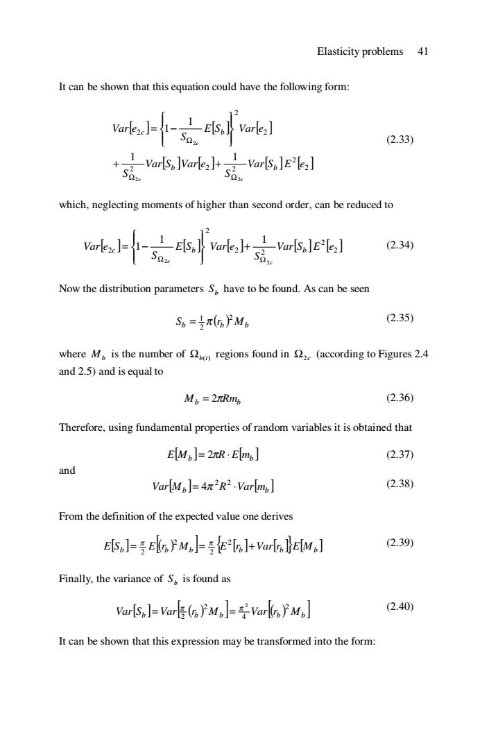
Elasticity problems 41 It can be shown that this equation could have the following form: okhf-云otkl (2.33) :-Var[S,]Varlez]+-2-Var[Sp]E2e2] which,neglecting moments of higher than second order,can be reduced to (2.34) Now the distribution parameters S,have to be found.As can be seen S6=号π(PMb (2.35) where M is the number of regions found in 2(according to Figures 2.4 and 2.5)and is equal to Mb=2πRmb (2.36) Therefore,using fundamental properties of random variables it is obtained that EMb]=2πR.Em%] (2.37) and VarMp]=4π2R2.Varm,] (2.38) From the definition of the expected value one derives ESJ=号Ek,PM=号E2]+arl}EMJ (2.39) Finally,the variance of S is found as Var[Sp]=Var(YMoJ=Var(oYMpJ (2.40) It can be shown that this expression may be transformed into the form:
Elasticity problems 41 It can be shown that this equation could have the following form: [ ] [] [] [ ] [] [ ] [] 2 2 2 2 2 2 2 2 2 2 2 1 1 1 1 Var S E e S Var S Var e S E S Var e S Var e b b c b c c c Ω Ω Ω + + ⎪⎭ ⎪ ⎬ ⎫ ⎪⎩ ⎪ ⎨ ⎧ = − (2.33) which, neglecting moments of higher than second order, can be reduced to [ ] [] [] [] [] 2 2 2 2 2 2 2 2 1 1 1 Var S E e S E S Var e S Var e c b b Ω c Ω c + ⎪⎭ ⎪ ⎬ ⎫ ⎪⎩ ⎪ ⎨ ⎧ = − (2.34) Now the distribution parameters b S have to be found. As can be seen ( ) b b Mb S r 2 2 1 = π (2.35) where Mb is the number of Ωb(i) regions found in Ω2c (according to Figures 2.4 and 2.5) and is equal to Mb πRmb = 2 (2.36) Therefore, using fundamental properties of random variables it is obtained that [ ] [] E Mb R E mb = 2π ⋅ (2.37) and [ ] [] Var Mb R Var mb = ⋅ 2 2 4π (2.38) From the definition of the expected value one derives [ ] [( ) ] { } [] [] [ ] b b b b b E Mb E S = E r M = E r +Var r 2 2 2 2 π π (2.39) Finally, the variance of Sb is found as Var[ ] Sb Var[ ( ) rb Mb ] Var[( ) rb Mb ] 2 4 2 2 2 π π = = (2.40) It can be shown that this expression may be transformed into the form:

42 Computational Mechanics of Composite Materials Var[Sp]==(E2[r]+Varlrp]Var[Mp] (2.41) +Varlol(E-[M,J+Var[M.DG2E-LJ+VartD Substituting the equations describing S distribution parameters into the relations describing the expected value and variance of the e,modulus,we can similarly derive the data necessary for numerical analysis. Using analogous equations,the stochastic interface defects in the fibre region can be approximated.So,let us assume a finite number of these discontinuities inserted into the contact zone.As already established,the fibre material has good resistance to degradation (much better than the matrix)and because of this,the defects in the region can be approximated as teeth with their sharp sides directed towards the fibre centre.A single discontinuity is,from the geometrical point of view,the superposition of two circular quadrants with the same radius (Figure 2.6).There holds a4云刺 (2.42) and ak小上太whl (2.43) 克vrtsvrs.le-6l X 2 Figure 2.6.Teeth interface defects in fibre-reinforced composite
42 Computational Mechanics of Composite Materials [ ] ( ) [] [] [ ] [] [ ] [ ] ( )( ) [] [] b b b b b b b b b Var r E M Var M E r Var r Var S E r Var r Var M + + + = + 2 2 2 2 2 4 2 2 2 π π (2.41) Substituting the equations describing b S distribution parameters into the relations describing the expected value and variance of the k e modulus, we can similarly derive the data necessary for numerical analysis. Using analogous equations, the stochastic interface defects in the fibre region can be approximated. So, let us assume a finite number of these discontinuities inserted into the contact zone. As already established, the fibre material has good resistance to degradation (much better than the matrix) and because of this, the defects in the Ω1 region can be approximated as teeth with their sharp sides directed towards the fibre centre. A single discontinuity is, from the geometrical point of view, the superposition of two circular quadrants with the same radius (Figure 2.6). There holds [ ] [ ]⎟ ⎟ ⎠ ⎞ ⎜ ⎜ ⎝ ⎛ = − Ω c t E S S E e E e 1c 1 [ ] 1 1 1 (2.42) and [ ] [ ] [] [ ] [] [ ] []1 2 2 1 2 1 2 1 1 1 1 1 1 1 1 Var S E e S Var S Var e S E S Var e S Var e t t c t c c c Ω Ω Ω + + ⎪⎭ ⎪ ⎬ ⎫ ⎪⎩ ⎪ ⎨ ⎧ = − (2.43) Figure 2.6. Teeth interface defects in fibre-reinforced composite
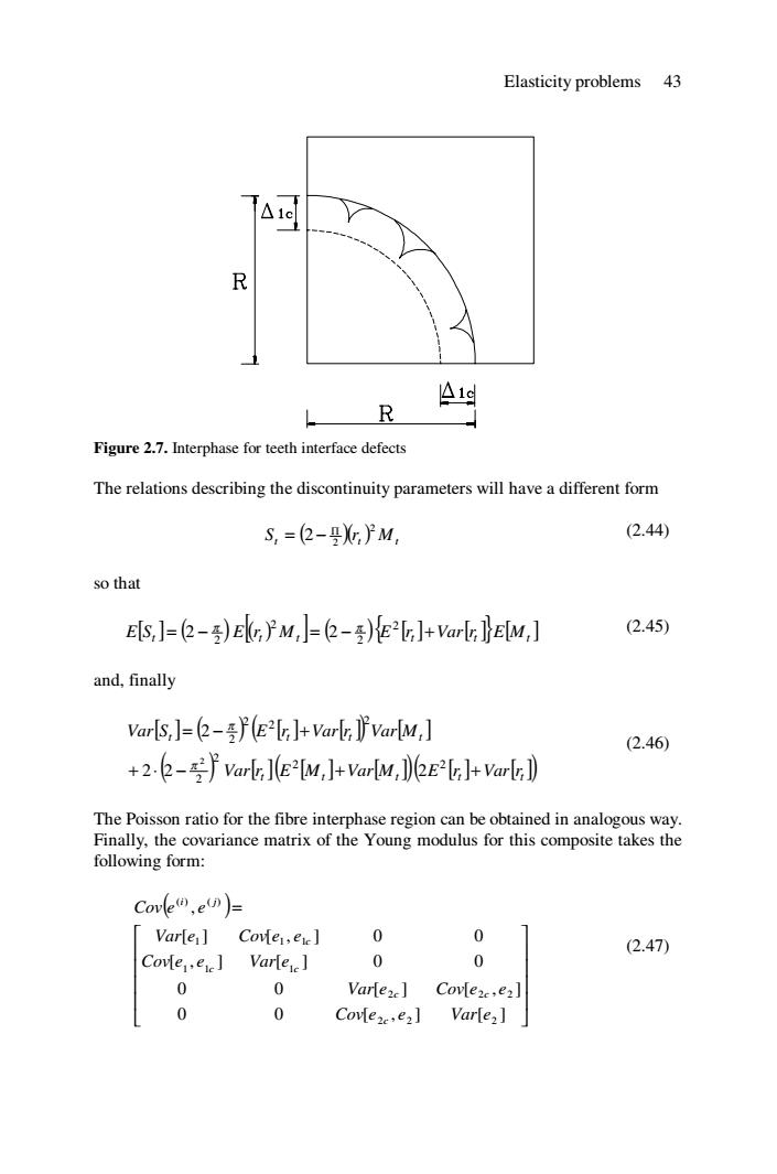
Elasticity problems 43 R A1d R Figure 2.7.Interphase for teeth interface defects The relations describing the discontinuity parameters will have a different form S,=(2-%}M, (2.44) so that E,]=-)Ek}M,]=-)Ee]+arL]}EM,] (2.45) and,finally Var[S,J=(2-(E2IrJ+Varlr]var[M,] (2.46) +2.-Varl](E-[M,J+Var[M,)(2E2LJ+Varlr] The Poisson ratio for the fibre interphase region can be obtained in analogous way. Finally,the covariance matrix of the Young modulus for this composite takes the following form: Covle,en))= Varle Cover,eve] 0 0 (2.47) Cove.ere]Varlee] 0 0 0 0 Varteze]Covleze,e2l 0 0 Cove2e.e2] Var[e2]
Elasticity problems 43 Figure 2.7. Interphase for teeth interface defects The relations describing the discontinuity parameters will have a different form ( )( ) t t Mt S r 2 2 2 Π = − (2.44) so that [ ] ( ) [( ) ] ( ){ } [] [] [ ] t t t t t E Mt E S = − E r M = − E r +Var r 2 2 2 2 2 2 π π (2.45) and, finally [ ] ( ) ( ) [] [] [ ] ( ) [] [ ] [ ] ( )( ) [] [] t t t t t t t t t Var r E M Var M E r Var r Var S E r Var r Var M + ⋅ − + + = − + 2 2 2 2 2 2 2 2 2 2 2 2 2 π π (2.46) The Poisson ratio for the fibre interphase region can be obtained in analogous way. Finally, the covariance matrix of the Young modulus for this composite takes the following form: ( ) ⎥ ⎥ ⎥ ⎥ ⎦ ⎤ ⎢ ⎢ ⎢ ⎢ ⎣ ⎡ = 0 0 [ , ] [ ] 0 0 [ ] [ , ] [ , ] [ ] 0 0 [ ] [ , ] 0 0 , 2 2 2 2 2 2 1 1 1 1 1 1 ( ) ( ) Cov e e Var e Var e Cov e e Cov e e Var e Var e Cov e e Cov e e c c c c c c i j (2.47)
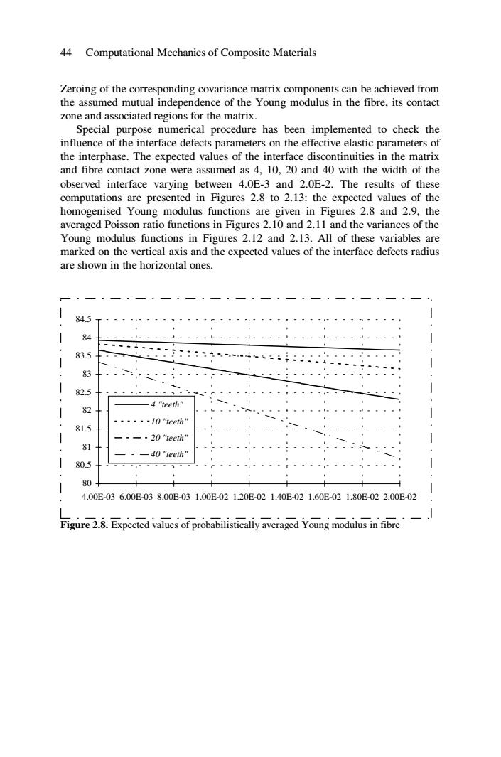
44 Computational Mechanics of Composite Materials Zeroing of the corresponding covariance matrix components can be achieved from the assumed mutual independence of the Young modulus in the fibre,its contact zone and associated regions for the matrix. Special purpose numerical procedure has been implemented to check the influence of the interface defects parameters on the effective elastic parameters of the interphase.The expected values of the interface discontinuities in the matrix and fibre contact zone were assumed as 4,10,20 and 40 with the width of the observed interface varying between 4.0E-3 and 2.0E-2.The results of these computations are presented in Figures 2.8 to 2.13:the expected values of the homogenised Young modulus functions are given in Figures 2.8 and 2.9,the averaged Poisson ratio functions in Figures 2.10 and 2.11 and the variances of the Young modulus functions in Figures 2.12 and 2.13.All of these variables are marked on the vertical axis and the expected values of the interface defects radius are shown in the horizontal ones. 84.5 84 83.5 83 82.5 -4 "teeth" 82 -····-0"1eeth" 81.5 -·20"1eeth" 81 -40 "teeth" 80.5 80 4.00E-036.00E-038.00E-031.00E-021.20E-021.40E-021.60E-021.80E-022.00E-02 Figure 2.8.Expected values of probabilistically averaged Young modulus in fibre
44 Computational Mechanics of Composite Materials Zeroing of the corresponding covariance matrix components can be achieved from the assumed mutual independence of the Young modulus in the fibre, its contact zone and associated regions for the matrix. Special purpose numerical procedure has been implemented to check the influence of the interface defects parameters on the effective elastic parameters of the interphase. The expected values of the interface discontinuities in the matrix and fibre contact zone were assumed as 4, 10, 20 and 40 with the width of the observed interface varying between 4.0E-3 and 2.0E-2. The results of these computations are presented in Figures 2.8 to 2.13: the expected values of the homogenised Young modulus functions are given in Figures 2.8 and 2.9, the averaged Poisson ratio functions in Figures 2.10 and 2.11 and the variances of the Young modulus functions in Figures 2.12 and 2.13. All of these variables are marked on the vertical axis and the expected values of the interface defects radius are shown in the horizontal ones. 80 80.5 81 81.5 82 82.5 83 83.5 84 84.5 4.00E-03 6.00E-03 8.00E-03 1.00E-02 1.20E-02 1.40E-02 1.60E-02 1.80E-02 2.00E-02 4 "teeth" 10 "teeth" 20 "teeth" 40 "teeth" Figure 2.8. Expected values of probabilistically averaged Young modulus in fibre