The Review of Financial Studies/v 10 n 3 1997 the associated distributional theory that the limiting distribution of √T(R-p)is normal. Even though the limiting distribution of the sample R2 under HA is normal,the fact that the R2 criterion is strictly nonnegative suggests that the rate of approach to normality is likely to be relatively slow. It should be possible to improve the approximation,however,by exploiting well-known small sample results.Consider,for example, the scenario where the sequence (1,represents an i.i.d.sample from a multivariate normal distribution.Anderson (1984)shows that in this case √T(-p)号N0,41-p)2). (12) The important thing to note about the distribution in Equation (12)is that the variance is a direct function of the population value of R2. As a result,the t-ratio for the sample R2 tends to exhibit substantial departures from normality in small samples.An easy way to improve the small sample performance under these circumstances is to perform a variance-stabilizing transformation. Suppose we let f(R2)denote the function In((1+R)/(1-R)), where R is the sample multiple-correlation coefficient for a one- period return horizon.It follows by application of the delta method that f(R)N(f(p )1/T). (13) Thus,the transformation yields an asymptotic distribution whose vari- ance is independent of the population value of R2.Because of this property,there is good reason to suspect that the t-ratio for f(R2)will perform better in small samples than will the t-ratio associated with the original distribution. Now take the more general scenario where the data can exhibit serial correlation,conditional heteroscedasticity,and nonnormalities. Although the above transformation may no longer achieve complete variance stabilization,it still has the potential to improve inferences about the magnitude of the population R2.The basic idea is as follows. First compute the quantity f(R2)=In((1+Re)/(1-Ra)).Then construct the standard error of f(R)using the delta method.The sample multiple correlation coefficient can be written as Re tanh(f(R)), (14) where tanh()denotes the hyperbolic tangent.Because the hyperbolic tangent is a monotonic transformation,it follows that an approximate (1-c)%confidence interval for the sample multiple correlation coef- 588
Measuring the Predictable Variation in Stock and Bond Returns ficient is tanh(f)-Φ(c/2)r)≤pe≤tanh(f(+Φ(c/2)r), (15) where (and or denote the cumulative distribution function of a standard normal random variable and the standard error of f(), respectively.4 2.Data and Econometric Methodology The data used for the empirical analysis mirrors that of Fama and French (1989).This choice of data is motivated by a simple consid- eration.The Fama and French article is one of the most widely cited studies of long-horizon predictability,so it makes sense to relate the current analysis directly to their work.The dataset is comprised of monthly holding period returns on portfolios of common stock and bonds.The data begin in January 1927 and end in December 1987 (732 observations).All portfolio returns are calculated in excess of the one-month return for the Treasury bill that is closest to 30 days to maturity.Excess returns for horizons exceeding one month are computed by cumulating monthly excess returns. 2.1 The portfolios The long-term predictability of common stock returns is evaluated using two different market indices:the equal-weighted and value- weighted portfolios constructed from all the firms listed on the New York Stock Exchange (NYSE).Return data for the two indices are pro- vided by the Center for Research in Security Prices(CRSP)at the Uni- versity of Chicago.The value-weighted index is skewed toward stocks that have a high market capitalization,while the equal-weighted index gives equal representation to all firms.Fama and French (1989)argue that these two portfolios provide a convenient way to study how firm size affects the ability to predict returns. The bond portfolio returns are drawn from a database maintained by Ibbotson Associates.This database contains monthly holding pe- riod returns on a number of different portfolios of corporate bonds. The five portfolios used in the empirical analysis are constructed from bonds rated Aaa,Aa,A,Baa,and below Baa (LG,low-grade) by Moody's.Bond portfolio returns are calculated by taking a price weighted average of the individual returns for the constituent bonds The average time to maturity of the bonds in each portfolio is typically greater than 10 years. 4 See Chapter 4 of Anderson (1984)for a discussion of this method of drawing inferences within the context of normal correlation theory. 589
The Review of Financial Studies/v 10 n 3 1997 2.2 The Instruments The instrumental variables used in the long-horizon regressions are the same as those used by Fama and French (1989),but the data used to construct the instruments are drawn from different sources.The first instrument is the dividend yield on the S&P composite stock index (D/V).Data on this instrument are obtained from Standard and Poor's Current Statistics.The second instrument is a term spread (TERM).It is calculated by subtracting the annualized yield on a one-month Trea- sury bill from the annualized yield on Moody's Aaa bond portfolio. The final instrument is a default risk spread (DEF).It is equal to the annualized yield on Moody's Baa bond portfolio minus the annual- ized yield on Moody's Aaa bond portfolio.The data used to construct both the term spread and the default risk spread are drawn from Moody's Industrial Manual.All three instruments are constructed us- ing monthly observations. Table 1 provides descriptive statistics for the excess returns and in- strumental variables.The statistics for the monthly observations are fa- miliar from other studies that use similar data.In general,the monthly stock and bond returns exhibit only a modest degree of serial cor- relation.The instrumental variables,on the other hand,are highly autocorrelated.Note that the first-order autocorrelation coefficient for both DIV and DEF exceeds 0.95.It appears,however,that the serial correlation of these two variables decays toward zero at a rate that is consistent with the view that each of the time series is stationary.The results for the annual data are similar. 2.3 The long-horizon regressions The key claim of Fama and French (1989)is that three instruments-a term spread,a default spread,and the dividend yield on the NYSE index-explain a large fraction of the variation in long-horizon stock and bond returns.This claim stems from the fact that when the portfo- lio returns are regressed on various combinations of the three instru- ments,the sample R2 increases from around 3%for monthly returns to well over 25%for four-year returns.Therefore,the first step is to replicate these regressions by estimating a linear model of the form 元+=a+(B十E+k (16) 5 Fama and French(1989)use the dividend yield on the NYSE index instead of the dividend yield on the S&P composite index,and their term spread and default spread are constructed from yield data maintained by Ibbotson Associates.The advantage of using the Moody's yield data is twofold. First,it is much more widely available than the Ibbotson data and has therefore been used in a number of well-known studies of predictability.Second,its use provides a good check on the general robustness of the Fama and French (1989)results. 590
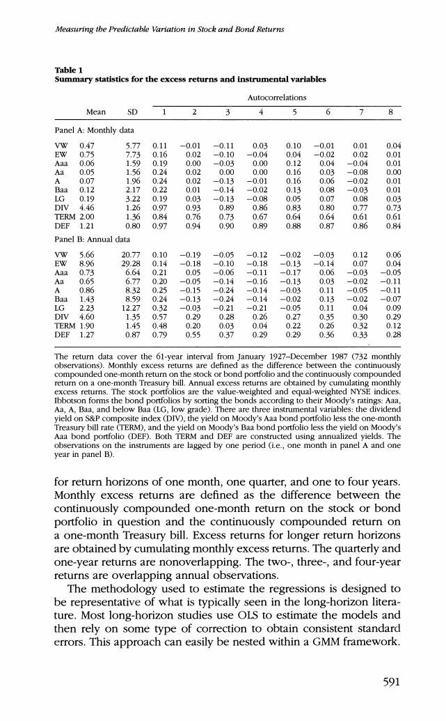
Measuring tbe Predictable Variation in Stock and Bond Returns Table 1 Summary statistics for the excess returns and instrumental variables Autocorrelations Mean SD 1 3 5 Panel A:Monthly data VW 0.47 5.77 0.11 -0.01 -0.11 0.03 0.10 -0.01 0.01 0.04 EW 0.75 7.73 0.16 0.02 -0.10 -0.04 0.04 -0.02 0.02 0.01 Aaa 0.06 1.59 0.19 0.00 -0.03 0.00 0.12 0.04 -0.04 0.01 Aa 0.05 1.56 0.24 0.02 0.00 0.00 0.16 0.03 -0.08 0.00 A 0.07 1.96 0.24 0.02 -0.13 -0.01 0.16 0.06 -0.02 0.01 Baa 0.12 2.17 0.22 0.01 -0.14 -0.02 0.13 0.08 -0.03 0.01 LG 0.19 3.22 0.19 0.03 -0.13 -0.08 0.05 0.07 0.08 0.03 DIV 4.46 1.26 0.97 0.93 0.89 0.86 0.83 0.80 0.77 0.73 TERM 2.00 1.36 0.84 0.76 0.73 0.67 0.64 0.64 0.61 0.61 DEF 1.21 0.80 0.97 0.94 0.90 0.89 0.88 0.87 0.86 0.84 Panel B:Annual data VW 5.66 20.77 0.10 -0.19 -0.05 -0.12 -0.02 -0.03 0.12 0.06 EW 8.96 29.28 0.14 -0.18 -0.10 -0.18 -0.13 -0.14 0.07 0.04 Aaa 0.73 6.64 0.21 0.05 -0.06 -0.11 -0.17 0.06 -0.03 -0.05 Aa 0.65 6.77 0.20 -0.05 -0.14 -0.16 -0.13 0.03 -0.02 -0.11 A 0.86 8.32 0.25 -0.15 -0.24 -0.14 -0.03 0.11 -0.05 -0.11 Baa 1.43 8.59 0.24 -0.13 -0.24 -0.14 -0.02 0.13 -0.02 -0.07 LG 2.23 12.27 0.32 -0.03 -0.21 -0.21 -0.05 0.11 0.04 0.09 DIV 4.60 1.35 0.57 0.29 0.28 0.26 0.27 0.35 0.30 0.29 TERM 1.90 1.45 0.48 0.20 0.03 0.04 0.22 0.26 0.32 0.12 DEF 1.27 0.87 0.79 0.55 0.37 0.29 0.29 0.36 0.33 0.28 The return data cover the 61-year interval from January 1927-December 1987 (732 monthly observations).Monthly excess returns are defined as the difference between the continuously compounded one-month return on the stock or bond portfolio and the continuously compounded return on a one-month Treasury bill.Annual excess returns are obtained by cumulating monthly excess returns.The stock portfolios are the value-weighted and equal-weighted NYSE indices Ibbotson forms the bond portfolios by sorting the bonds according to their Moody's ratings:Aaa Aa,A,Baa,and below Baa (LG,low grade).There are three instrumental variables:the dividend yield on S&P composite index (DIV),the yield on Moody's Aaa bond portfolio less the one-month Treasury bill rate (TERM),and the yield on Moody's Baa bond portfolio less the yield on Moody's Aaa bond portfolio (DEF).Both TERM and DEF are constructed using annualized yields.The observations on the instruments are lagged by one period (i.e.,one month in panel A and one year in panel B). for return horizons of one month,one quarter,and one to four years. Monthly excess returns are defined as the difference between the continuously compounded one-month return on the stock or bond portfolio in question and the continuously compounded return on a one-month Treasury bill.Excess returns for longer return horizons are obtained by cumulating monthly excess returns.The quarterly and one-year returns are nonoverlapping.The two-,three-,and four-year returns are overlapping annual observations. The methodology used to estimate the regressions is designed to be representative of what is typically seen in the long-horizon litera- ture.Most long-horizon studies use OLS to estimate the models and then rely on some type of correction to obtain consistent standard errors.This approach can easily be nested within a GMM framework 591
The Review of Financial Studies/v 10 n 3 1997 Consider,for example,an econometric specification based on the dis- turbance vector, h(e,) ,i+-a- (∑1i+-e-B, (17) whereand =This disturbance vector contains the OLS normal equations.Because the econometric system in Equation (17)is exactly identified,the GMM estimator of 0 is the value that sets 1/T)equal to zero.It is easy to see that this value is obtained by replacing each element of the vector e with its sample analog.The sample analog of the vector B is the least-squares estimator B&,so the estimates of the slope coefficients obtained using the GMM procedure are identical to those that result from fitting a multiple regression model to the data. 2.4 Tests for predictability Tests of the null hypothesis that returns are unpredictable are con- structed based on the limiting distribution of the GMM estimator.6 This distribution takes the form √T(©-)4N(0,(D'S-1D)-1), (18) where D=E 3h(0) 80 and S= Eh(e,8)h(e-,θ)1.(19) If 0 is partitioned as [e02 where 02=B and the matrix (D'S-D)-1 is partitioned accordingly,then the Wald statistic, wo=T(022z2a2) (20) converges to a chi-square random variable with m degrees of freedom under the null hypothesis that returns are unpredictable.It is shown in the Appendix that n2z is the V matrix of Theorem 1.1.Although V is generally unknown,it can be replaced by a consistent estimator without affecting the limiting distribution of the test statistic. Computing the GMM estimator of the slope coefficients is straight- forward,but the approach used to construct the variance-covariance 6 In the discussion that follows it is assumed that is generated by a stationary,ergodic process and that the second moment matrix of h()exists and is finite.This assumption,along with the regularity conditions given by Hansen (1982),is sufficient for the asymptotic distribution theory of GMM to hold. 592