Measuring the Predictable Variation in Stock and Bond Returns model shown in Equation (1)are stochastic,the least-squares estima- tor of the vector of slope coefficients is given by ae=26, (2) wheredenotes the sample analog of the variance-covariance ma- trix of the instruments,and z denotes the m x 1 vector of sample covariances.The limiting distribution of the least-squares estimator is provided by the following theorem. Theorem 1.1.Let(n,be a stationary and ergodic process.Furtber assume that the regularity conditions given by Hansen (1982)are satisfied.Then the limiting distribution of the least-squares estimator ofF。is √T(3。-B)号N(0,V, (3) wbere T denotes the number of observations in the data set.The variance-covariance matrix V is given by 2z2 (④ wbere=(-aB),and u:denotes the ex- pected value of the vector i:. It certainly comes as no surprise that the limiting distribution of the least-squares estimator is multivariate normal.But one feature of the distribution in Equation (3)deserves close attention.Note how the autocovariance structure of the disturbance vector=(-) affects the variance-covariance matrix of the estimator.This relation is important because the matrix V plays a large role in determining the limiting distribution of the sample R2.To see why,recall that the sample R can be written as a quadratic form in the least-squares estimator of the vector of slope coefficients.If serial correlation or heteroscedasticity make it impossible to obtain a precise estimate of Ba,then the sample R2 will reflect a similar degree of imprecision. Thus,the statistical properties of the disturbance vector n+have a The sample R2 is equal to the sample variance of the fitted values divided by the sample variance of the dependent variable.Applying this definition to the model shown in Equation (1)yields: where denotes the sample variance of the k-period excess return on the portfolio. 583
The Review of Financial Studies /v 10 n 3 1997 great deal to do with the distributional properties of the sample R2 One of the goals of this article is to develop formal theoretical results that clearly illustrate this relation.A natural first step in this process is to consider the case where the assumptions of classical regression analysis are satisfied. 1.2 Serially uncorrelated homoscedastic disturbances Let the null hypothesis Ho be that asset returns are unpredictable.In addition,assume that the disturbance vectorn is serially uncorre- lated and that is conditionally homoscedastic.2 Within the context of the regression model shown in Equation (1),the testable implica- tion of the null is that B=0.When we impose the null hypothesis and incorporate the stated assumptions,the limiting distribution of the sample R2 takes the form given in the following theorem. Tbeorem 1.2.Let (r,be a stationary and ergodic process.Furtber assume that the regularity conditions of Hansen (1982)are satisfied, that cov(n+e,i+e-t)=0 for all卡0,and that var(i+k)=o2∑zz, wbere og denotes the variance f.Then,under the null bypothesis Ho,the limiting distribution of the sample R2 for the model shown in Equation (1)is TR4X玩 (5) wbere X denotes a central cbi-square distribution with m degrees of freedom. It is not difficult to see why the quantity TR is asymptotically dis- tributed as a chi-square random variable.Under the conditions stated in the theorem,the matrix V in Equation (4)reduces to,where o denotes the variance of the k-period excess return.As a result,the Wald statistic for testing the null hypothesis is 6 (6) where 2 denotes the sample analog of o2.Once the ratio inside the parentheses is recognized as the sample R2 for the regression model of Equation (1),the distributional results of Theorem 1.2 follow immediately.3 2 One scenario consistent with this assumption is that is serially uncorrelated and distributed independently of for all i. 3 It is well known that,under the null hypothesis,the Wald statistic in Equation (6)converges in distribution to a chi-square random variable with m degrees of freedom. 584
Measuring the Predictable Variation in Stock and Bond Returns The asymptotic results shown in Equations (5)and (6)bear a dis- tinct resemblance to the small sample results for the multivariate nor- mal regression model.This similarity stems in large part from the as- sumption that (i)is serially uncorrelated;and (ii)the error term for the regression model is conditionally homoscedastic.In situations where these assumptions are plausible,the sample R2 represents an appealing criterion for evaluating whether the null hypothesis of no predictability is credible.To obtain significance points for the sample R2,we simply divide the values for the appropriate chi-square dis- tribution by the number of observations used in the analysis.If the observed value of the sample R2 exceeds the cutoff,then the null hypothesis that asset returns are unpredictable is rejected.It is impor- tant to keep in mind,of course,that tests performed in this manner are valid only if the aforementioned restrictions on and are satisfied.The effect of relaxing these restrictions is considered in Sec- tion 1.3. 1.3 Autocorrelated heteroscedastic disturbances Stock and bond returns are known to exhibit a marked degree of conditional heteroscedasticity,and overlapping returns are autocor- related by construction.As a consequence,the sampling theory for long-horizon models must be able to accommodate both serial cor- relation and conditional heteroscedasticity of unknown form.If the previous analysis is modified to permit the sorts of intertemporal de- pendence and conditional heterogeneity that may exist in data gener- ated by a stationary and ergodic process,then the limiting distribution of the sample R2 under null hypothesis Ho takes the form given in Theorem 1.3. Theorem 1.3.Let (,be a stationary and ergodic process.Furtber assume that the regularity conditions given by Hansen (1982)are satisfied.In addition,allowk and to exbibit the type of serial correlation and conditional beteroscedasticity that is consistent with data generated by a stationary and ergodic process.Then,under the null bypotbesis Ho,the limiting distribution of the sample R2 for the model sbown in Equation (1)is TRQ. (7) wbere Q denotes the general distribution of a quadratic form in a multivariate normal random vector.The mean and variance of O are ug≡tr(o62V∑zz) and 0g=2r(o62V∑zz)2, (8) wbere tr()denotes the trace operator. 585
The Review of Financial Studies/v 10n 3 1997 Given the results of Theorem 1.3,the potential consequences of serial correlation and conditional heteroscedasticity begin to emerge more clearly.First,consider the traditional scenario whereis seri- ally uncorrelated and is conditionally homoscedastic.Under the null,the v matrix in Equation (8)is given by so the mean and variance of o are equal to m and 2m,the values for a chi-square distribution with m degrees of freedom.Now let the disturbances display serial correlation and/or conditional heteroscedasticity,and notice how the analysis changes.One difference,of course,is that the matrix V becomes more complex and the results grow less ana- lytically tractable.More importantly,though,the mean and variance of o take on values that may be far removed from those of a chi- square distribution.This shift in the mean and variance of the limiting distribution of TR suggests a possible explanation for reports that long-horizon returns are highly predictable. Studies that examine long-horizon predictability typically use in- strumental variables that are highly persistent.The combination of highly persistent instruments and overlapping returns induces strong serial correlation in the least-squares disturbance vector.As a result, the OLS standard errors for the model understate the variance of the least-squares estimator of the slope coefficients.Although researchers have long recognized that the OLS t-ratios are unreliable in long- horizon regressions,many fail to make the connection between in- flated t-ratios and the sample R2.The easiest way to illustrate the relation is to consider a long-horizon model with a single regressor. In this case,the sample R2 can be written asts/(1+),where tols denotes the OLS t-ratio for a test of the null hypothesis that the least- squares estimator of the slope coefficient is equal to zero.It stands to reason,therefore,that if the OLS t-ratio is inflated,then the sample R2 will also be misleading. The intuition for the single-regressor case carries over to the multi- ple regression setting as well.If the OLS t-ratios are misleading under the null,then the researcher has a clear signal that the traditional interpretation of the sample R2 is no longer valid.One potential so- lution to this problem is to use the limiting distribution given in The- orem 1.3 to test whether the sample R2is significantly different from zero.Unfortunately,this strategy is not really practical given the com- plex nature of the distribution in question.There is,however,a related approach that can be implemented quite easily.First,use standard, large-sample,chi-square tests to evaluate whether the null hypothesis of no predictability is credible.In the event that such tests indicate a rejection of the null,then the limiting distribution of the sample R under the alternative hypothesis can be used to draw inferences about the size of the predictable component of returns.The limiting distri- 586
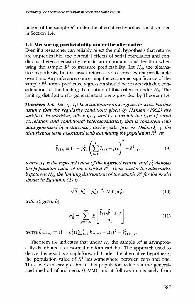
Measuring the Predictable Variation in Stock and Bond Returns bution of the sample R2 under the alternative hypothesis is discussed in Section 1.4. 1.4 Measuring predictability under the alternative Even if a researcher can reliably reject the null hypothesis that returns are unpredictable,the potential effects of serial correlation and con- ditional heteroscedasticity remain an important consideration when using the sample R2 to measure predictability.Let HA,the alterna- tive hypothesis,be that asset returns are to some extent predictable over time.Any inference concerning the economic significance of the sample R2 from a predictive regression should be drawn with due con- sideration for the limiting distribution of this criterion under H4.The limiting distribution for general situations is provided by Theorem 1.4. Tbeorem 1.4.Let(r,i)be a stationary and ergodic process.Furtber assume that the regularity conditions given by Hansen (1982)are satisfied.In addition,allowk and exbibit the type of serial correlation and conditional beteroscedasticity that is consistent with data generated by a stationary and ergodic process.Define k the disturbance term associated with estimating the population R-,as 5+≡(1-p哈) (- (9) wbere uk is the expected value of the k-period return,and pdenotes the population value of the k-period R2.Then,under the alternative bypotbesis HA,the limiting distribution of the sample R-for the model shown in Equation (1)is √T(R路-)号N0,o), (10) with o given by E (11) 0bere专+k-j=(1-p爱(∑17+i--ue)2-品+k- Theorem 1.4 indicates that under Ha the sample R2 is asymptoti- cally distributed as a normal random variable.The approach used to derive this result is straightforward.Under the alternative hypothesis, the population value of R2 lies somewhere between zero and one. Thus,we can easily estimate this population value via the general- ized method of moments (GMM),and it follows immediately from 587