
1.2.Probability Density of a Region R If we assume that p(x)is continuous and the region R is small enough that p(x) has little change in the R region,then we can get an approximation as follows: P=pxx≈p6r where x is a point in R and V is the volume of this region of R(V is the area in 2D) From Pk/n,the probability density function of R region can be approximated as: 10/45
1.2. Probability Density of a Region R ▶ If we assume that p(x) is continuous and the region R is small enough that p(x) has little change in the R region, then we can get an approximation as follows: P = Z R p(x ′ )dx′ ≈ p(x)V where x is a point in R and V is the volume of this region of R (V is the area in 2D). ▶ From P ≈ k/n, the probability density function of R region can be approximated as: p(x) ≈ P V ≈ k/n V 10 / 45
p)≈ n Its validation depends on two contradictory assumptions: 1 Region R be sufficiently small that the density is approximately constant over the region 2 Region R be sufficiently large(in relation to the value of that density)that the number k of samples falling inside the region is sufficient for the binomial distribution to be sharply peaked. Condition of converging to the true probability density in the limit noo, 1 Ishrinks suitably with n 2 k grows with n 11/45
p(x) ≈ k/n V ▶ Its validation depends on two contradictory assumptions: 1 Region R be sufficiently small that the density is approximately constant over the region 2 Region R be sufficiently large (in relation to the value of that density) that the number k of samples falling inside the region is sufficient for the binomial distribution to be sharply peaked. ▶ Condition of converging to the true probability density in the limit n → ∞, 1 V shrinks suitably with n 2 k grows with n 11 / 45
px)¥ k n V In practice,we will have to find a compromise for V: 1 Large enough to include enough examples within R 2 Small enough to support the assumption that is constant within R Two ways to calculate p(x): fix Iand determine k from the data,giving rise to the kernel approach,such as histogram,Parzen window 2 fix k and determine Ifrom the data,which gives rise to the k-nearest neighbors 12/45
p(x) ≃ k/n V ▶ In practice, we will have to find a compromise for V: 1 Large enough to include enough examples within R 2 Small enough to support the assumption that is constant within R ▶ Two ways to calculate p(x): 1 fix V and determine k from the data, giving rise to the kernel approach, such as histogram, Parzen window 2 fix k and determine V from the data, which gives rise to the k-nearest neighbors 12 / 45

Outline (Level 1) Density Estimation 2 Histogram Method Parzen Window k-nearest neighbors Summary of nonparametric models 13/45
Outline (Level 1) 1 Density Estimation 2 Histogram Method 3 Parzen Window 4 k-nearest neighbors 5 Summary of nonparametric models 13 / 45
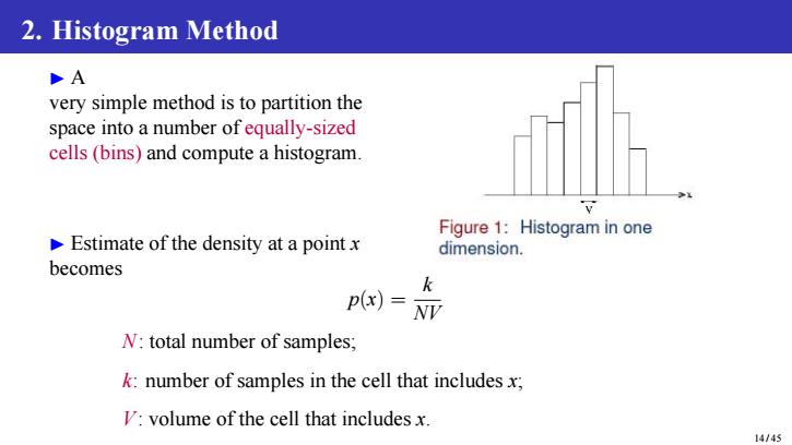
2.Histogram Method DA very simple method is to partition the space into a number of equally-sized cells(bins)and compute a histogram. Figure 1:Histogram in one Estimate of the density at a pointx dimension. becomes k p(x) N:total number of samples; k:number of samples in the cell that includes x; V:volume of the cell that includes x. 14/45
2. Histogram Method ▶ A very simple method is to partition the space into a number of equally-sized cells (bins) and compute a histogram. ▶ Estimate of the density at a point x becomes p(x) = k NV N: total number of samples; k: number of samples in the cell that includes x; V: volume of the cell that includes x. 14 / 45