Chapter 1 Presenting and Summarizing Data 1.1 Data and Variables Data are the material with which statisticians work.They are records of measurement, counts or observations.Examples of data are records of weights of calves.milk vield in lactation of a gr oup of cows ale or female sex.and blue or g een color of eyes.A set of observations on a particular char cter is termed a variable.For example.variables denoting the data listed above are weight.milk yield.sex.and eye color.Data are the values of a variable.for exam ple,a weight of 200 kg.a daily milk yield of 20 kg. male.or blue eyes. The expression variable de icts that measurements or observations can be different,i.e. they show variability.Variables can be defined as quantitative (numerical)and qualitative (attributive,categorical,or classification). Quantitative variables have values expressed as numbers and the differences between values have numerical meaning.Examples of quantitative variables are weight of animals, litter size,temperature or time.They also can include ratios of two numerical variables. count data.and proportions.A quantitative variable can be continuous or discrete.A continuous variable can take on an infinite number of values over a given interval.Its values are real numbers.A discrete variable is a variable that has countable values,and the number of those values can either be finite or infinite.Its values are natural numbers or integers. Examples of continuous variables are milk yield or weight,and examples of discrete variables are litter size or number of laid eggs per month. Qualitative variables have values expressed in categories.Examples of qualitative variables are eye color or whether or not an animal is ill.A qualitative variable can be an ordinal or nominal.An ordinal variable has categories that can be ranked.A nominal variable has categories that cannot be ranked.No category is more valuable than another. Examples of nominal variables are identification number,color or gender,and an example of an ordinal variable is calving ease scoring.For example,calving ease can be described in 5 categories,but those categories can be enumerated:1.normal calving.2.calving with little intervention,3.calving with considerable intervention,4.very difficult calving,and 5. Caesarean section.We can assign numbers (scores)to ordinal categories;however,the differences among those numbers do not have numerical meaning.For example,for calving ease,the difference between score I and 2 (normal calving and calving with little intervention)does not have the same meaning as the difference between 4 and 5(very difficult calving and Caesarean section).As a rule those scores depict categories,but not a numerical scale.On the basis of the definition of a qualitative variable it may be possible to assign some quantitative variables,for example,the number of animals that belong to a category,or the proportion of animals in one category out of the total number of animals. 1
1 Chapter 1 Presenting and Summarizing Data 1.1 Data and Variables Data are the material with which statisticians work. They are records of measurement, counts or observations. Examples of data are records of weights of calves, milk yield in lactation of a group of cows, male or female sex, and blue or green color of eyes. A set of observations on a particular character is termed a variable. For example, variables denoting the data listed above are weight, milk yield, sex, and eye color. Data are the values of a variable, for example, a weight of 200 kg, a daily milk yield of 20 kg, male, or blue eyes. The expression variable depicts that measurements or observations can be different, i.e., they show variability. Variables can be defined as quantitative (numerical) and qualitative (attributive, categorical, or classification). Quantitative variables have values expressed as numbers and the differences between values have numerical meaning. Examples of quantitative variables are weight of animals, litter size, temperature or time. They also can include ratios of two numerical variables, count data, and proportions. A quantitative variable can be continuous or discrete. A continuous variable can take on an infinite number of values over a given interval. Its values are real numbers. A discrete variable is a variable that has countable values, and the number of those values can either be finite or infinite. Its values are natural numbers or integers. Examples of continuous variables are milk yield or weight, and examples of discrete variables are litter size or number of laid eggs per month. Qualitative variables have values expressed in categories. Examples of qualitative variables are eye color or whether or not an animal is ill. A qualitative variable can be an ordinal or nominal. An ordinal variable has categories that can be ranked. A nominal variable has categories that cannot be ranked. No category is more valuable than another. Examples of nominal variables are identification number, color or gender, and an example of an ordinal variable is calving ease scoring. For example, calving ease can be described in 5 categories, but those categories can be enumerated: 1. normal calving, 2. calving with little intervention, 3. calving with considerable intervention, 4. very difficult calving, and 5. Caesarean section. We can assign numbers (scores) to ordinal categories; however, the differences among those numbers do not have numerical meaning. For example, for calving ease, the difference between score 1 and 2 (normal calving and calving with little intervention) does not have the same meaning as the difference between 4 and 5 (very difficult calving and Caesarean section). As a rule those scores depict categories, but not a numerical scale. On the basis of the definition of a qualitative variable it may be possible to assign some quantitative variables, for example, the number of animals that belong to a category, or the proportion of animals in one category out of the total number of animals
2 Biostatistics for Animal Science 1.2 Graphical Presentation of Qualitative Data When describing qualitative data each observation is assigned to a specific category.Data are then described by the number of observations in each category or by the proportion of the total number of observations.The frequency for a certain category is the number of observations in that category.The relative frequency for a certain category is the proportion of the total number of observations.Graphical presentations of qualitative variables can include bar,column or pie-charts. Example:The numbers of cows in Croatia under milk recording by breed are listed in the following table: Breed Number of cows Percentage Simmental 62672 76% Holstein-Friesiar 15195 19% Brown 3855 5% Total 81722 100% The number of cows can be presented using bars with each bar representing a breed (Figure1.1). 855 Holstein 15195 mmenta 2672 0 20000400006000080000 Number of cows Figure 1.1 Number of cows under milk recording by breed The proportions or percentage of cows by breed can also be shown using a pie-chart (Figure 1.2)
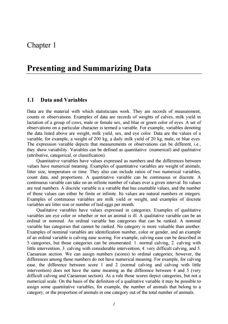
2 Biostatistics for Animal Science 1.2 Graphical Presentation of Qualitative Data When describing qualitative data each observation is assigned to a specific category. Data are then described by the number of observations in each category or by the proportion of the total number of observations. The frequency for a certain category is the number of observations in that category. The relative frequency for a certain category is the proportion of the total number of observations. Graphical presentations of qualitative variables can include bar, column or pie-charts. Example: The numbers of cows in Croatia under milk recording by breed are listed in the following table: Breed Number of cows Percentage Simmental 62672 76% Holstein-Friesian 15195 19% Brown 3855 5% Total 81722 100% The number of cows can be presented using bars with each bar representing a breed (Figure 1.1). 62672 15195 3855 0 20000 40000 60000 80000 Simmental Holstein Brown Breed Number of cows Figure 1.1 Number of cows under milk recording by breed The proportions or percentage of cows by breed can also be shown using a pie-chart (Figure 1.2)
Chapter I Presenting and Summarizing Data 3 % 19% Figure 1.2 Percentage of cows under milk recording by breed 1.3 Graphical Presentation of Quantitative Data The most widely used graph for presentation of quantitative data is a histogram.A histogram is a frequency distribution of a set of data.In order to present a distribution,the quantitative data are partitioned into classes and the histogram shows the number or relative frequency of observations for each class. 1.3.1 Construction of a Histogram Instructions for drawing a histogram can be listed in several steps: 1.Caleu late the range:(Range=maximum-minimum value) 2.Divide the range into five to 20 classes,depending on the number of observations.The class width is obtained by rounding the result up to an integer number.The lowest class boundary must be defined below the minimum value,the highest class boundary must be defined above the maximum value. 3.For each class,count the number of observations belonging to that class.This is the true calculated by dividing the tru by the total number of ency/total number of servations). (o bar)grap with class boundaries
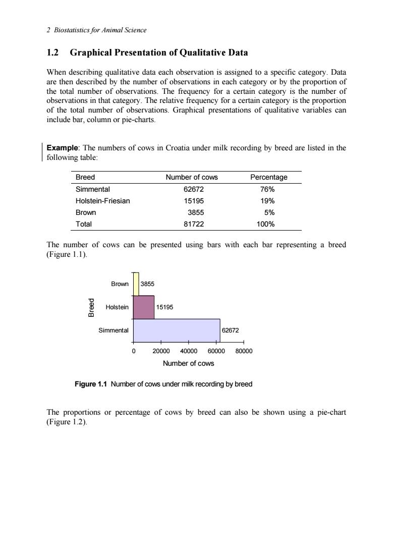
Chapter 1 Presenting and Summarizing Data 3 Simmental 76% Holstein 19% Brown 5% Figure 1.2 Percentage of cows under milk recording by breed 1.3 Graphical Presentation of Quantitative Data The most widely used graph for presentation of quantitative data is a histogram. A histogram is a frequency distribution of a set of data. In order to present a distribution, the quantitative data are partitioned into classes and the histogram shows the number or relative frequency of observations for each class. 1.3.1 Construction of a Histogram Instructions for drawing a histogram can be listed in several steps: 1. Calculate the range: (Range = maximum – minimum value) 2. Divide the range into five to 20 classes, depending on the number of observations. The class width is obtained by rounding the result up to an integer number. The lowest class boundary must be defined below the minimum value, the highest class boundary must be defined above the maximum value. 3. For each class, count the number of observations belonging to that class. This is the true frequency. 4. The relative frequency is calculated by dividing the true frequency by the total number of observations: (Relative frequency = true frequency / total number of observations). 5. The histogram is a column (or bar) graph with class boundaries defined on one axis and frequencies on the other axis
4 Biostatistics for Animal Science Example:Construct a histogram for the 7-month weights (kg)of 100 calves: 233 208 306 300 271 304 207 254 262 231 279 228 287 223 247 292 209 303 194 263 262 234 277 291 256 271 255 269 278 290 259 251 265 316 318 252 316 221 249 304 241 249 289 211 273 241 215 264 216 271 196 269 236 320 245 244 239 6 255 8 245 255 329 240 262 291 275 272 218 317 251 257 327 222 227 251 266 255 214 304 230 250 Minimum=194 Maximum 329 Range=329-194=135 For a total 15 classes,the width of a class is: 135/15=9 The class width can be rounded to 10 and the following table constructed: Class Class Number of Relative Cumulative limits midrange calves Frequency(%)number of calves 185.194 190 1 1 1 195-204 200 1 2 205-214 210 5 5 > 215-224 220 8 8 15 225-234 230 8 8 23 235-244 240 6 6 29 245-254 250 12 41 255-264 260 6 16 57 265-274 270 12 12 69 275-284 280 7 76 285-294 290 7 83 295-304 300 8 8 305.314 310 2 2 3 315-324 320 98 325-334 330 2 2 100 Figure 1.3 presents the histogram of weights of calves.The classes are on the horizonta axis and the numbers of animals are on the vertical axi Class values are expressed as the class midranges(midpoint between the limits),but could alternatively be expressed as class limits
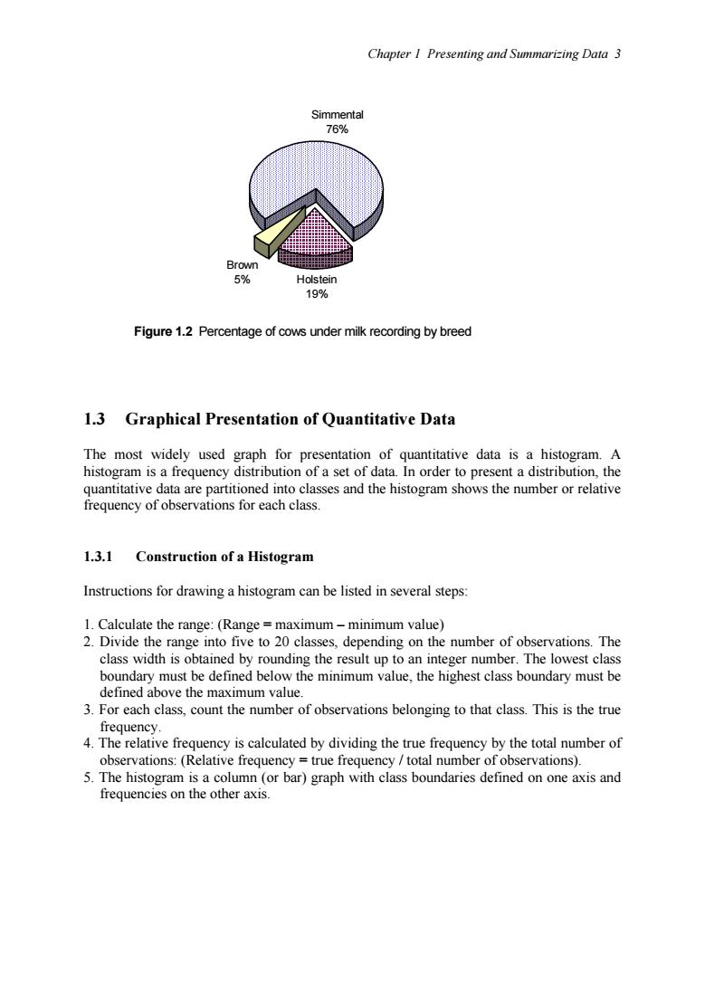
4 Biostatistics for Animal Science Example: Construct a histogram for the 7-month weights (kg) of 100 calves: 233 208 306 300 271 304 207 254 262 231 279 228 287 223 247 292 209 303 194 268 263 262 234 277 291 277 256 271 255 299 278 290 259 251 265 316 318 252 316 221 249 304 241 249 289 211 273 241 215 264 216 271 296 196 269 231 272 236 219 312 320 245 263 244 239 227 275 255 292 246 245 255 329 240 262 291 275 272 218 317 251 257 327 222 266 227 255 251 298 255 266 255 214 304 272 230 224 250 255 284 Minimum = 194 Maximum = 329 Range = 329 - 194 = 135 For a total 15 classes, the width of a class is: 135 / 15 = 9 The class width can be rounded to 10 and the following table constructed: Class limits Class midrange Number of calves Relative Frequency (%) Cumulative number of calves 185 - 194 190 1 1 1 195 - 204 200 1 1 2 205 - 214 210 5 5 7 215 - 224 220 8 8 15 225 - 234 230 8 8 23 235 - 244 240 6 6 29 245 - 254 250 12 12 41 255 - 264 260 16 16 57 265 - 274 270 12 12 69 275 - 284 280 7 7 76 285 - 294 290 7 7 83 295 - 304 300 8 8 91 305 - 314 310 2 2 93 315 - 324 320 5 5 98 325 - 334 330 2 2 100 Figure 1.3 presents the histogram of weights of calves. The classes are on the horizontal axis and the numbers of animals are on the vertical axis. Class values are expressed as the class midranges (midpoint between the limits), but could alternatively be expressed as class limits
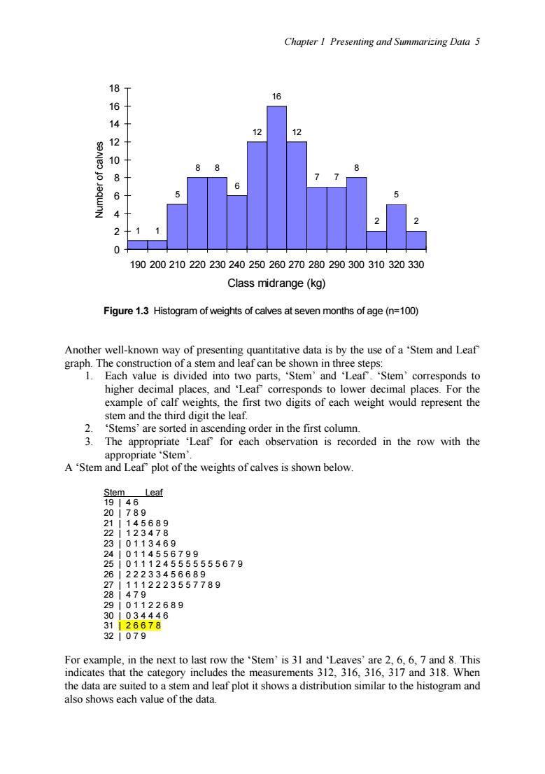
Chapter I Presenting and Summarizing Data 5 181 16 14 10 8 1 2 190200210220230240250260270280290300310320330 Class midrange(kg) Figure 1.3 Histogram of weights of calves at seven months of age(n=100) well-kn own way of present data is by the use of a'Stem and Leaf graph. can be wn id "Ste three esp al mple places.Fo stem and the leaf The approp Leaf fo is recorded in the row with the plot of the weights of calves is shown below Ster Leaf 2 489 2 12589日 3458789 355 011124555 555679 12223557789 122689 28676 321079 t row the 363567 This 31 whe ta are su d eshments32316” ribution similar to the histogram and
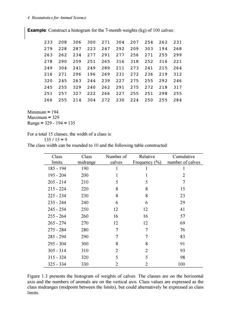
Chapter 1 Presenting and Summarizing Data 5 1 1 5 8 8 6 12 16 12 7 7 8 2 5 2 0 2 4 6 8 10 12 14 16 18 190 200 210 220 230 240 250 260 270 280 290 300 310 320 330 Class midrange (kg) Number of calves Figure 1.3 Histogram of weights of calves at seven months of age (n=100) Another well-known way of presenting quantitative data is by the use of a ‘Stem and Leaf’ graph. The construction of a stem and leaf can be shown in three steps: 1. Each value is divided into two parts, ‘Stem’ and ‘Leaf’. ‘Stem’ corresponds to higher decimal places, and ‘Leaf’ corresponds to lower decimal places. For the example of calf weights, the first two digits of each weight would represent the stem and the third digit the leaf. 2. ‘Stems’ are sorted in ascending order in the first column. 3. The appropriate ‘Leaf’ for each observation is recorded in the row with the appropriate ‘Stem’. A ‘Stem and Leaf’ plot of the weights of calves is shown below. Stem Leaf 19 | 4 6 20 | 7 8 9 21 | 1 4 5 6 8 9 22 | 1 2 3 4 7 8 23 | 0 1 1 3 4 6 9 24 | 0 1 1 4 5 5 6 7 9 9 25 | 0 1 1 1 2 4 5 5 5 5 5 5 5 6 7 9 26 | 2 2 2 3 3 4 5 6 6 8 9 27 | 1 1 1 2 2 2 3 5 5 7 7 8 9 28 | 4 7 9 29 | 0 1 1 2 2 6 8 9 30 | 0 3 4 4 4 6 31 | 2 6 6 7 8 32 | 0 7 9 For example, in the next to last row the ‘Stem’ is 31 and ‘Leaves’ are 2, 6, 6, 7 and 8. This indicates that the category includes the measurements 312, 316, 316, 317 and 318. When the data are suited to a stem and leaf plot it shows a distribution similar to the histogram and also shows each value of the data