6 Computational Mechanics of Composite Materials if only the Lesbegue integral with respect to the probabilistic measure exists and converges. Lemma Eel=e (1.21) Lemma There holds for any random numbers X and the real numbers c,E (1.22) Lemma There holds for any independent random variables X ex.-fex.] (1.23) Definition Let us consider the following random variable X:defined on the probabilistic space (F,P).The variance of the variable X is defined as Var(X)=[(X(@)-E[X]YdP(@) (1.24) Q and the standard deviation is called the quantity G(X)=Var(X) (1.25) Lemma 女Var(c)=0 (1.26 Lemma Y Var(cX)=c-Var(X) (1.27) E Lemma There holds for any two independent random variables X and Y Var(X +Y)=Var(X)+Var(Y) (1.28) Var(X.Y)=E[X].Var(Y)+Var(X).Var(Y)+Var(X).E[Y] (1.29)
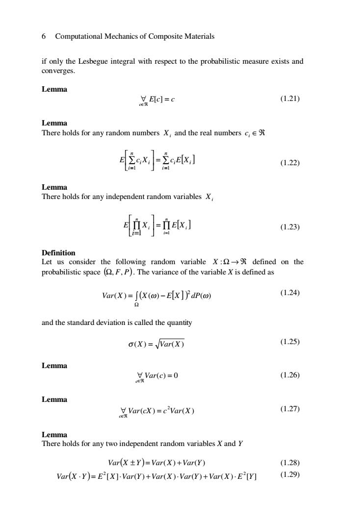
6 Computational Mechanics of Composite Materials if only the Lesbegue integral with respect to the probabilistic measure exists and converges. Lemma E c c c ∀ = ∈ℜ [ ] (1.21) Lemma There holds for any random numbers Xi and the real numbers ci ∈ℜ ∑ ∑ [ ] = = =⎥ ⎦ ⎤ ⎢ ⎣ ⎡ n i i i n i E ci Xi c E X 1 1 (1.22) Lemma There holds for any independent random variables Xi ∏ ∏ [ ] = ⎥ = ⎦ ⎤ ⎢ ⎣ ⎡ = n i i n i E X i E X 1 1 (1.23) Definition Let us consider the following random variable X :Ω → ℜ defined on the probabilistic space ( ) Ω, F, P . The variance of the variable X is defined as ( ) [ ] ∫ Ω ( ) = ( ) − ( ) 2 Var X X ω E X dP ω (1.24) and the standard deviation is called the quantity σ (X) = Var(X ) (1.25) Lemma ∀ ( ) = 0 ∈ℜ Var c c (1.26) Lemma ( ) ( ) 2 Var cX c Var X c ∀ = ∈ℜ (1.27) Lemma There holds for any two independent random variables X and Y Var( ) X ± Y = Var(X) +Var(Y) (1.28) ( ) [ ] ( ) ( ) ( ) ( ) [ ] 2 2 Var X ⋅Y = E X ⋅Var Y +Var X ⋅Var Y +Var X ⋅ E Y (1.29)

Mathematical Preliminaries 7 Definition Let us consider the random variable X:defined on the probabilistic space (2,F,P).A complex function of the real variable o:Z such that p(t)=Eexp(itx】 (1.30) stands for the characteristic function of the variable X. 1.1.2 Gaussian and Quasi-Gaussian Random Variables Let us consider the random variable X having a Gaussian probability distribution function with m being the expected value and o >0 the standard deviation.The distribution function of this variable is (1.31) where the probability density function is calculated as f)= exp (r-m)2 202 (1.32) The characteristic function for this variable is denoted as o(t)=Elexp(itx)]=exp(mit-2). (1.33) If the variable X with the parameters(m,o)is Gaussian,then its linear transform Y=AX +B with A,Be is Gaussian,too,and its parameters are equal to Am+B and Ao for A≠0,respectively. Problem Let us consider the random variable X with the first two moments E[X]and Var(X). Let us determine the corresponding moments of the new variable Y=X2. Solution The problem has been solved using three different ways illustrating various methods applicable in this and in analogous cases.The generality of these methods make them available in the determination of probabilistic moments and their parameters for most random variables and their transforms for given or unknown
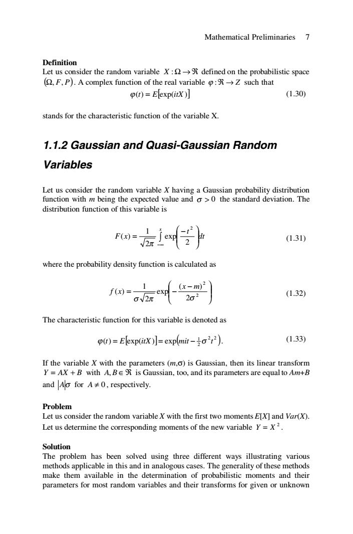
Mathematical Preliminaries 7 Definition Let us consider the random variable X :Ω → ℜ defined on the probabilistic space ( ) Ω, F, P . A complex function of the real variable ϕ :ℜ → Z such that ϕ(t) = E[ ] exp(itX ) (1.30) stands for the characteristic function of the variable X. 1.1.2 Gaussian and Quasi-Gaussian Random Variables Let us consider the random variable X having a Gaussian probability distribution function with m being the expected value and 0 σ > the standard deviation. The distribution function of this variable is dt t F x x ∫ −∞ ⎟ ⎟ ⎠ ⎞ ⎜ ⎜ ⎝ ⎛ − = 2 exp 2 1 ( ) 2 π (1.31) where the probability density function is calculated as ⎟ ⎟ ⎠ ⎞ ⎜ ⎜ ⎝ ⎛ − = − 2 2 2 ( ) exp 2 1 ( ) σ π σ x m f x (1.32) The characteristic function for this variable is denoted as [ ] ( ) 2 2 2 1 ϕ(t) = E exp(itX ) = exp mit − σ t . (1.33) If the variable X with the parameters (m,σ) is Gaussian, then its linear transform Y = AX + B with A, is Gaussian, too, and its parameters are equal to B ∈ℜ Am+B and Aσ for 0 A ≠ , respectively. Problem Let us consider the random variable X with the first two moments E[X] and Var(X). Let us determine the corresponding moments of the new variable 2 Y = X . Solution The problem has been solved using three different ways illustrating various methods applicable in this and in analogous cases. The generality of these methods make them available in the determination of probabilistic moments and their parameters for most random variables and their transforms for given or unknown

8 Computational Mechanics of Composite Materials probability density functions of the input frequently takes place in which numerous engineering problems. I method Starting from the definition of the variance of a ny random variable one can write Var(Y)=E(Y2)-E2(Y) (1.34) Let Y=X2,then Var(X2)=E(X2)2)-E2(X2) (1.35) The value of E will be determined through integration of the characteristic function for the Gaussian probability density function (1.36) where m=E[X]and o=Var(X)denote the expected value and standard deviation of the considered distribution,respectively.Next,the following standardised variable is introduced t=x-m,where x=to+m,dx=adt (1.37) which gives k了+mreu叫} (1.38) After some algebraic transforms of the integrand function it is obtained that Ek☆了(or+4onmn户+6anm+4omr+me号h (1.39) and,dividing into particular integrals,there holds Ek]应oh+4oml,+6o2m21,+4om14+m1,)e号 (1.40) where the components denote
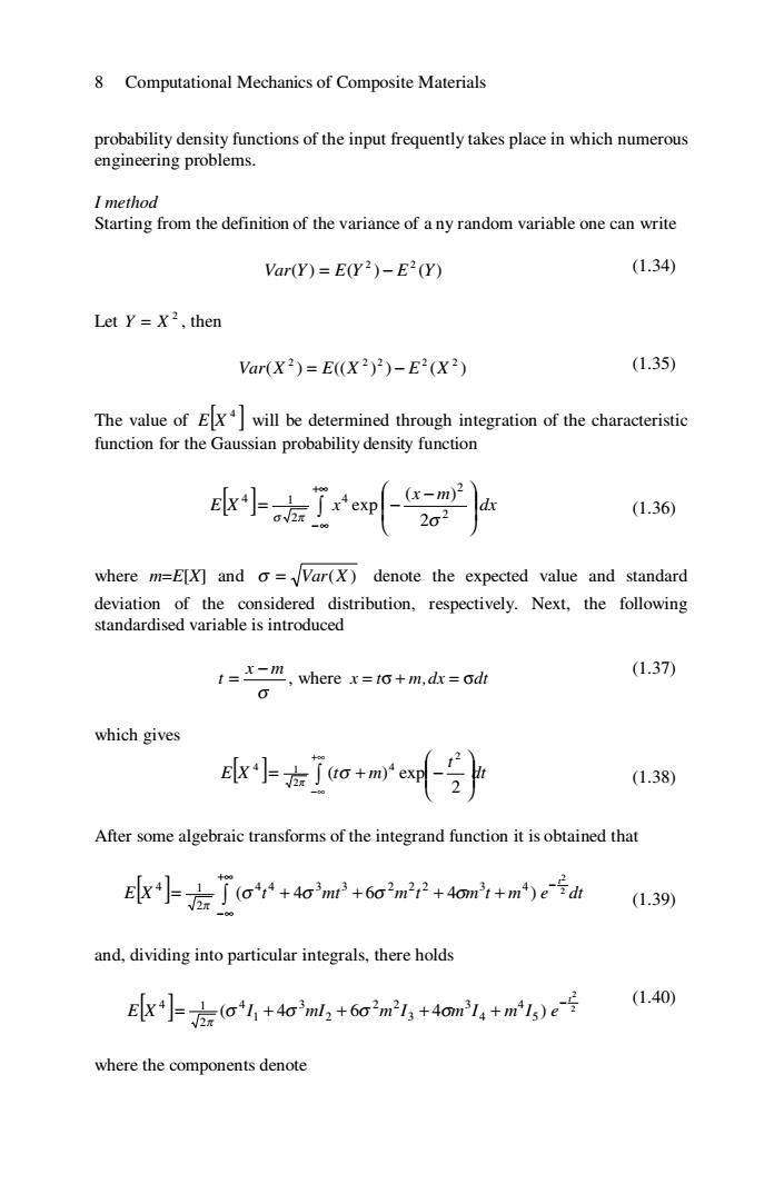
8 Computational Mechanics of Composite Materials probability density functions of the input frequently takes place in which numerous engineering problems. I method Starting from the definition of the variance of a ny random variable one can write ( ) ( ) ( ) 2 2 Var Y = E Y − E Y (1.34) Let 2 Y = X , then ( ) (( ) ) ( ) 2 2 2 2 2 Var X = E X − E X (1.35) The value of [ ] 4 E X will be determined through integration of the characteristic function for the Gaussian probability density function [ ] ∫ +∞ −∞ ⎟ ⎟ ⎠ ⎞ ⎜ ⎜ ⎝ ⎛ − = − dx x m E X x 2 2 4 2 4 1 2 ( ) exp σ π σ (1.36) where m=E[X] and σ = Var(X ) denote the expected value and standard deviation of the considered distribution, respectively. Next, the following standardised variable is introduced σ x m t − = , where x = tσ + m,dx = σdt (1.37) which gives [ ] dt t E X ∫ t m +∞ −∞ ⎟ ⎟ ⎠ ⎞ ⎜ ⎜ ⎝ ⎛ = + − 2 ( ) exp 2 4 2 4 1 σ π (1.38) After some algebraic transforms of the integrand function it is obtained that E[ ] X t mt m t m t m e dt t ∫ +∞ −∞ − = + + + + 2 2 ( 4 6 4 ) 4 4 3 3 2 2 2 3 4 2 4 1 σ σ σ σ π (1.39) and, dividing into particular integrals, there holds [ ] 2 2 ( 4 6 4 ) 5 4 4 3 3 2 2 2 3 1 4 2 4 1 t E X I mI m I m I m I e − = σ + σ + σ + σ + π (1.40) where the components denote

Mathematical Preliminaries 9 1,=jre号d:l,=jre9d;l,=jre号d: (1.41) I=jted:Is=jed It should be mentioned that the values of the odd integrals on the real domain are equal to 0 in the following calculation jf(x)g(x)dx-jf()g(dx+jf(x)g(x)d (1.42) If the function fx)is odd and g(x)is even x)=-fx),g(x)=g(x), (1.43) then it can be written jrd--d--d (1.44) Considering that the odd indices integrals are calculated;this results in 1,=je片di=际 (1.45) 5=rah=-了eh=-de5, (1.46) ∫e d=V2 4a-了-. (1.47) =-a-[-w际 After simplification the result is Ex4]=30+602m2+m=E+[X ]+6Var(X)E2[X]+3Var2(X) (1.48) Ex2=o2+m2=E2[X]+Var(X) (1.49)
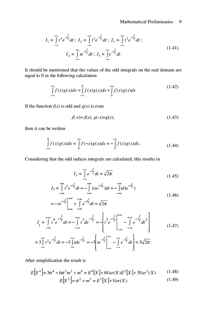
Mathematical Preliminaries 9 I t e dt t ∫ +∞ −∞ − = 2 2 4 1 ; I t e dt t ∫ +∞ −∞ − = 2 2 3 2 ; I t e dt t ∫ +∞ −∞ − = 2 2 2 3 ; I te dt t ∫ +∞ −∞ − = 2 2 4 ; I e dt t ∫ +∞ −∞ − = 2 2 5 (1.41) It should be mentioned that the values of the odd integrals on the real domain are equal to 0 in the following calculation ∫ ∫ ∫ +∞ −∞ +∞ −∞ = + 0 0 f (x)g(x)dx f (x)g(x)dx f (x)g(x)dx (1.42) If the function f(x) is odd and g(x) is even f(-x)=-f(x), g(-x)=g(x), (1.43) then it can be written ∫ ∫ ∫ +∞ +∞ −∞ = − = − 0 0 0 f (x)g(x)dx f ( x)g(x)dx f (x)g(x)dx . (1.44) Considering that the odd indices integrals are calculated; this results in 2π 2 2 5 = ∫ = +∞ −∞ − I e dt t (1.45) 2π ( ) ( ) 2 2 2 2 2 2 2 2 2 2 2 3 = − + = = = − = − ∫ ∫ ∫ ∫ +∞ −∞ − +∞ −∞ − − +∞ −∞ +∞ −∞ − +∞ −∞ − te e dt I t e dt t te dt td e t t t t t (1.46) ⎥ ⎥ ⎥ ⎦ ⎤ ⎢ ⎢ ⎢ ⎣ ⎡ = ∫ = − ∫ = − − ∫ +∞ −∞ − +∞ −∞ − − +∞ −∞ +∞ −∞ 4 − 3 3 3 1 2 2 2 2 2 2 2 2 I t e dt t de t e e dt t t t t 3 3 3 3 2π 2 2 2 2 2 2 2 2 2 = ⎥ ⎥ ⎦ ⎤ ⎢ ⎢ ⎣ ⎡ = ∫ = − ∫ = − − ∫ +∞ −∞ − +∞ −∞ − − +∞ −∞ +∞ −∞ − t e dt tde te e dt t t t t . (1.47) After simplification the result is [ ] 3 6 [] [] 6 ( ) 3 ( ) 4 4 2 2 4 4 2 2 E X = σ + σ m + m = E X + Var X E X + Var X (1.48) [ ] [ ] ( ) 2 2 2 2 E X = σ + m = E X +Var X (1.49)

10 Computational Mechanics of Composite Materials Var(x3=E4E2k2=2o2(o2+2m2) (1.50) =2Var(X)(Var(X)+2E2[X) IⅡnethod Initial algebraic rules can be proved following the method shown below.Using a modified algebraic definition of the variance Var(x2)=Ex-E2x*] (1.51) and the expected value Elx2]=Var(X)+E"[x] (1.52) subtracted from the following equation E2x=(Var(X)+E2[x]=Var2x+2Var(X)E2[x]+E[x] (1.53) we can demonstrate the following desired result: Var(X2)=EX-Var2(X)-2Var(X)E2[X]-E[X] (1.54) III method The characteristic function for the Gaussian PDF has the following form: p()=exp(mit--o2r2)】 (1.55) where p(0=*Ex}5k≥0 (1.56 and =(0)=im (1.57) The mathematical induction rule leads us to the conclusion that pm)=m-to2pm-(0-(0n-1o2.pa-2》0),n≥2 (1.58) which results in the equations
10 Computational Mechanics of Composite Materials [ ] [ ] 2 ( )( ( ) 2 [ ]) ( ) 2 ( 2 ) 2 2 4 2 2 2 2 2 Var X Var X E X Var X E X E X m = + = − = σ σ + (1.50) II method Initial algebraic rules can be proved following the method shown below. Using a modified algebraic definition of the variance [] [] 2 4 2 2 Var(X ) = E X − E X (1.51) and the expected value E[X ] Var X E [ ] X 2 2 = ( ) + (1.52) subtracted from the following equation E [ ] X ( ) Var X E [ ] X Var X Var X E [] [] X E X 2 2 4 2 2 2 2 = ( ) + = + 2 ( ) + (1.53) we can demonstrate the following desired result: Var X E[X ] Var X Var X E X E [ ] X 2 4 2 2 4 ( ) = − ( ) − 2 ( ) [ ] − (1.54) III method The characteristic function for the Gaussian PDF has the following form: ( ) 2 2 2 1 ϕ(t) = exp mit − σ t (1.55) where [ ] k k k (0) = i E X ( ) ϕ ; k ≥ 0 (1.56) and ϕ = ϕ (0) ; ϕ′(0) = im (1.57) The mathematical induction rule leads us to the conclusion that ( ) ( ) ( ) ( 1) ( ) ( ) 2 ( 1) 2 ( 2) t im t t n t n n− n− ϕ = − σ ⋅ϕ − − σ ⋅ϕ , 2 n ≥ (1.58) which results in the equations