
An Anatomy of Trading Strategies 1.The Profitability of Trading Strategies We consider a set of trading strategies that either explicitly mimic or capture the essence of previously implemented strategies.Specifically,consider buying or selling stocks at time t-I based on their performance from time t-2 to t-1,where the period (t-1,t]spans any finite time interval. Also,assume that the "performance"of a stock is determined relative to the average performance of all stocks that are used in the trading strategy. Consequently,if the entire universe of assets is included in the strategy,then each stock's performance is measured relative to the return on the equal- weighted"market portfolio,"Rm.Finally,let wir-I denote the fraction of the trading strategy portfolio devoted to security i [see Lehmann(1990)and Lo and MacKinlay (1990)],that is, w1-1k)=±R-1k-Rm-1k)】 (1) where Ri-(k)is the return on security i at time t-1,i 1,....N, R-1(k)is the return on equal-weighted portfolio of all securities,and k is the length of the time-interval {t-1,t). Since the weights are based entirely on information at time t-1,wi- has a subscript of t-1.The expression for the weights in Equation(1)suc- cinctly captures the philosophy of all return-based trading strategies.First, the positive or negative sign preceding the expression on the right-hand side reflects an investor's (institution's)beliefs;that is,whether the investor be- lieves in price continuations or reversals(and therefore recommends and/or follows a momentum or a contrarian strategy).Second,it is important to note that,regardless of whether a strategy is contrarian or momentum,the premise is that its success is based on the time-series behavior of asset prices.Specifically,a security's past performance relative to some bench- mark (e.g.,the average return of the portfolio of all securities)is supposed to be informative about future innovations in the security's prices.This is quite contrary,for example,to the random walk model of stock prices which implies that changes in stock prices are completely unpredictable (see Section 2 for further details).Third,the dollar weights in Equation(1) [i.e.,w-(k),...,wN-1(k)]lead to an arbitrage (zero cost)portfolio by construction Wit-1(k)=0 Yk, (2a) and the dollar investment long(or short)is given by w-1(k) (2b) 493
The Review of Financial Studies /v 1I n 3 1998 Fourth,since the weights in Equation (1)are proportional to the ab- solute value of the deviations of a security's return from the return of an equal-weighted portfolio of all securities,they capture the general belief that extreme price movements are followed by extreme movements [see, e.g.,DeBondt and Thaler (1985),Lehmann (1990),Lo and MacKinlay (1990),and Jegadeesh and Titman (1993)].Finally,and most importantly, the weights in Equation (1)allow us to conveniently decompose the prof- its of the trading strategies [see Lehmann(1990)and Lo and MacKinlay (1990)],again regardless of the inherent nature of the strategy (i.e.,whether it is a contrarian or a momentum strategy).This,in turn,permits us to determine the relative importance of the different components.2 The realized profits at time t,,(k),to the trading strategies implied by the weights in Equation(1)are given by N π,(k)=) wit-1(k)Rir(k) (3) i=l Since all the strategies considered in this article (and typically in the literature)are zero-cost strategies,only the dollar profits(and not the returns) are defined as in Equation(3).And if the markets are frictionless,the weights can be arbitrarily scaled to obtain any level of profits.We therefore will largely rely on the sign and statistical significance of the averages of the time series of the ,(k)'s;that is,we examine whether expected profits are statistically significantly positive (or negative). Table 1 contains average/expected profits for trading strategies imple- mented during different time periods and for different holding periods(i.e., different k).We consider five time periods:1962-1989;1926-1989,and three equal-size subperiods within the 1926-1989 period (January 1926- April 1947,May 1947-August 1968,September 1968-December 1989) We first implement the strategies for the 1962-1989 period because it cor- responds with the time period used in several past studies [see,e.g.,Lehmann (1990),Lo and MacKinlay (1990),and Jegadeesh and Titman(1993)].The 1926-1989 period is used (for all but the weekly holding period)because it covers a much longer time interval,and this interval (and the subperiods within it)provide a robustness check for the potential profitability of trading strategies. We use eight different holding periods k,where k ranges from I week 2 Jegadeesh and Titman(1993)use a variant of this strategy in which securities are ranked based on their past performance and are then combined into 10 portfolios that are held for a specific period of time.An arbitrage portfolio is also formed by buying the top performers and selling the worst performers.They note that the correlation between the returns to the strategy used in this article and their work is 0.95; however,the profits of their strategy cannot be readily decomposed.We follow the weighting scheme implied in Equation(1)instead,especially since a decomposition of the profits is central to this article. The weights in Equation(1),however,do retain the same philosophy as the other return-based strategy. 494
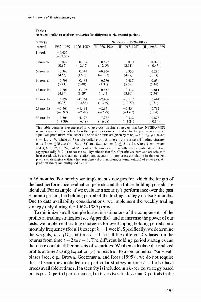
An Anatomy of Trading Strategies Table 1 Average profits to trading strategies for different horizons and periods Strategy Subperiods(1926-1989) interval 1962-19891926-1989 ()1926-1946(11)1947-1967(11)1968-1989 I week -0.035 (-23.30) 3 months 0.027 -0.165 -0.557 0.070 -0.020 (0.67) (-2.42) (-2.99) (2.91) (-0.43) 6 months 0.360 0.147 -0.204 0.333 0.273 (4.55) (1.91) (-1.03) (4.97) (3.63) 9 months 0.708 0.488 0.276 0.487 0.634 (5.81) (5.48) (I.37) (5.09) (5.44) 12 months 0.701 0.198 -0.557 0.372 0.611 (4.64) (1.29) (-1.44) (3.80) (3.70) 18 months 0.094 -0.761 -2.466 -0.117 0.444 (0.35) (-2.88) (-3.49) (-0.77) (1.51) 24 months -0.501 -1.181 -2.831 -0.434 0.792 (-0.97) (-2.98) (-2.92) (-1.62) (1.54) 36 months -3.304 -4.176 -7.727 -0.922 -0.873 (-3.39) (-6.48) -6.08) (-1.24) (-0.84) This table contains average profits to zero-cost trading strategies that buy NYSE/AMEX winners and sell losers based on their past performance relative to the performance of an equal-weighted index of all stocks.The dollar profits are given by (k)=w()R(k) i=1.....N,where (k)is the dollar profit at time t from a k-period trading strategy, war1(k)=[R-1(k)-Rm-1(k)]and Rw1(k)=Ri1(k).wherek I week. and 3,6.9.12.18.24.and 36 months.The numbers in parentheses are z-statistics that are asymptotically N(0.1)under the null hypothesis that"true"profits are zero and are robust to heteroscedasticity and autocorrelation,and account for any cross-correlation in the realized profits of strategies within a horizon class(short,medium.or long horizon)of strategies.All profit estimates are multiplied by 100. to 36 months.For brevity we implement strategies for which the length of the past performance evaluation periods and the future holding periods are identical.For example,if we evaluate a security's performance over the past 3-month period,the holding period of the trading strategy is also 3 months. Due to data availability considerations,we implement the weekly trading strategy only during the 1962-1989 period. To minimize small-sample biases in estimators of the components of the profits of trading strategies(see Appendix),and to increase the power of our tests,we implement trading strategies for overlapping holding periods on a monthly frequency(for all k exceptk I week).Specifically,we determine the weights,wir-1(k),at time t-I for all the different k's based on the returns from time t-2 to t-1.The different holding period strategies can therefore contain different sets of securities.We then calculate the realized profits at time t using Equation(3)for each k.To avoid potential"survival" biases [see,e.g.,Brown,Goetzmann,and Ross(1995)],we do not require that all securities included in a particular strategy at time t-I also have prices available at time t.If a security is included in ak-period strategy based on its past k-period performance,but it survives for less than k periods in the 495
The Review of Financial Studies/v 11 n 3 1998 future (because it is delisted),we use a (k-j)period return in calculating (k),where i is the period of delisting.The estimates in Table I are the time-series averages,for each k,of the profits at each time t,(k). Finally,since the profits of momentum(contrarian)strategies are exactly equal to the losses of contrarian(momentum)strategies [see Equations (1) and (3)],we implement only momentum strategies (i.e.,we use the weights Wit1=+[Ri-1(k)-Rmt-1(k)]k).Consequently,a positive (nega- tive)estimate in Table 1 implies that on average a momentum(contrarian) strategy is profitable. Table 1 also contains the z-statistics in parentheses to test the statistical significance of the average profits (losses);these statistics are asymptoti- cally N(0,1)under the null hypothesis that the "true"profits are zero.We use a generalized method of moments [see Hansen (1982)]procedure to calculate standard errors.This procedure takes into account cross-sectional correlations(within a particular time period)in the realized profits of multi- ple strategies within the medium-and long-term classes,as well providing standard errors that are robust to heteroscedasticity and autocorrelation. Several interesting features of the profitability of trading strategies emerge from an inspection of Table 1.First,the number of positive and negative estimates of average profits are exactly the same;18 versus 18.Therefore, unconditionally,momentum and contrarian strategies are equally likely to be successful (at least based on the 36 strategies evaluated in Table 1).This finding is noteworthy given that momentum and contrarian strategies are (as noted in the introduction)diametrically opposed in philosophy. Second,21 of the 36 trading strategies are statistically significantly prof- itable;again the number of statistically significant contrarian versus mo- mentum strategies is approximately the same,II versus 10,respectively. Third,once we condition on the return horizon and/or the time period,how- ever,the similarities between contrarian and momentum trading strategies disappear.Specifically,there is a systematic relation between the horizon of the strategy and the trading philosophy that appears to"work."A momen- tum strategy is usually profitable at the medium(3-to 12-month)horizons: of the 20 medium-term strategies reported in Table 1,a momentum strategy is profitable in 15 of the cases.More importantly,all 11 of the momen- tum strategies that yield statistically significant profits are medium-horizon strategies.To gauge the success of the momentum strategy at the medium horizon,we test for the joint significance of the 3-to 12-month strategies within each time period.Not surprisingly,there is strong evidence that the medium-horizon momentum strategy is profitable in all time periods ex- cept the 1926-1947 subperiod:the chi-square statistics for each of the other four time periods have p-values of zero.During the 1926-1947 subperiod, however,a contrarian strategy is successful at the medium horizon;the chi- square statistic for the joint significance of the 3-to 12-month strategies has a p-value of 0.016. 496
An Anatomy of Trading Strategies On the other hand,the success of contrarian strategies is dependent on one subperiod,1926-1947.Of the 10 contrarian strategies that earn statis- tically significant profits,four occur in the 1926-1947 period and they are also responsible for the statistical significance of the contrarian profits of four more strategies in the overall 1926-1989 period.More significantly,a contrarian strategy is statistically profitable only twice in the three postwar subperiods.We again conduct statistical tests for the joint significance of the long-term (18-to 36-month)contrarian strategies.The chi-square statistic for the 1926-1989 period strongly supports the profitability of the long-run contrarian strategy with a p-value of zero,but this evidence is dependent on one time interval,the 1926-1947 subperiod.While the p-value for the chi-square statistic is 0.009 for the 1926-1947 subperiod,it is 0.193 for the 1948-1968 subperiod and 0.203 for the 1969-1989 period.3 Hence,the net profitability of the contrarian strategy is limited to the long-run and to the pre-1947 data.This evidence is also consistent with the results of Fama and French(1988)and Kim,Nelson,and Startz(1991),who find that long-term mean reversion in the prices of portfolios of securities is peculiar to the prewar period.Finally,although a contrarian strategy is obviously profitable at the weekly horizon in the 1962-1989 period,recent research shows that the profitability of short-term strategies may be spurious because it is generated by market microstructure biases.4 The most convincing evidence in Table I consequently is in favor of the momentum strategy,which provides support to proponents of the momen- tum strategy,both on Wall Street and among academicians [see,e.g.,As- ness (1994),Grinblatt,Titman,and Wermers (1994),Jegadeesh and Titman (1993,1995a),and Levy (1967);Hendricks,Patel,and Zeckhauser (1993) provide related evidence].For example,in the most recent study on trad- ing strategies,Jegadeesh and Titman(1993)implement 32 different 3-to 12-month momentum strategies over the 1962-1989 period and find each one to be profitable.Also,Grinblatt,Titman,and Wermers (1994)show that about 77%of the 155 mutual funds in their sample follow momentum We reestimate all the average profits in Table I conditional on the behavior of the market,that is,we regress the realized profits on the market return in excess of the risk-free rate.The alphas of these regressions are typically similar to the unconditional average profits reported in Table 1.For example,apart from rendering the average profits of the 12-month momentum strategy statistically significant,the average estimates of the profits of all other strategies and their statistical significance remain largely unchanged for the overall 1926-1989 period.During the subperiods.the only notable difference is that the 24-and 36-month contrarian strategies in the 1947-1967 subperiod and the 36-month strategy in the 1968-1989 subperiod yield statistically significant conditional profits.This last result provides some support for the Ball,Kothari,and Shanken (1995)finding that risk-adjusted contrarian profits are higher relative to the raw profits in the postwar period. 4Market microstructure effects (e.g.,the bid-ask bounce and inventory effects)present in transaction returns can explain significant proportions of the price reversals that lead to the apparent success of short-term contrarian strategies [see Jegadeesh and Titman(1995b)and Conrad.Gultekin,and Kaul (1997)].Any remaining profits to these short-term strategies disappear at low levels of transaction costs even for large institutional investors [see Bessembinder and Chan (1994)and Conrad,Gultekin,and Kaul (1997)1. 497