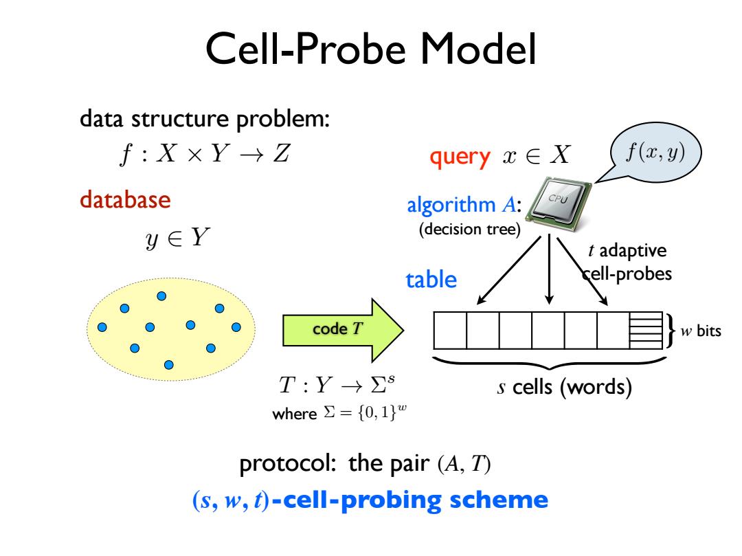
Cell-Probe Model data structure problem: f:X×Y→☑ query x∈X f(x,y) database algorithm A: CPU y∈Y (decision tree) t adaptive table cell-probes code T w bits T:Y→∑s s cells (words) where∑={0,1}w protocol:the pair (A,T) (s,w,t)-cell-probing scheme
code T table query x 2 X t adaptive cell-probes Cell-Probe Model } w bits ( s cells (words) algorithm A: ⌃ = {0, 1}w where (decision tree) protocol: the pair (A, T) database y 2 Y T : Y ! ⌃s f : X ⇥ Y ! Z data structure problem: (s, w, t)-cell-probing scheme f(x, y)
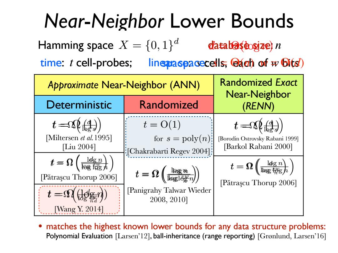
Near-Neighbor Lower Bounds Hamming space X ={0,1]d databaseosize)n time:t cell-probes;linepaspacecells;each of w bits) Approximate Near-Neighbor (ANN) Randomized Exact Near-Neighbor Deterministic Randomized (RENN) t=得) t=0(1) t=单 [Miltersen et al.1995] for s poly(n) Borodin Ostrovsky Rabani 1999] Liu2004] [Chakrabarti Regev 2004] Barkol Rabani 2000] Idg n 1og宽九 t=2 ldg n g玲照五 Patrascu Thorup 2006] t=() Patrascu Thorup 2006] t=刃 Panigrahy Talwar Wieder 2008,2010] Wang Y.2014] matches the highest known lower bounds for any data structure problems: Polynomial Evaluation [Larsen'12],ball-inheritance(range reporting)[Gronlund,Larsen'16]
Approximate Near-Neighbor (ANN) Randomized Exact Near-Neighbor Deterministic Randomized (RENN) Near-Neighbor Lower Bounds Hamming space X = {0, 1}d database size: n time: t cell-probes; space: s cells, each of w bits t = ⌦ ⇣ d log s ⌘ [Miltersen et al.1995] [Liu 2004] t = ⌦ ⇣ d log sw n ⌘ [Pătraşcu Thorup 2006] t = ⌦ ⇣ d log sw nd ⌘ [Wang Y. 2014] t = ⌦ ⇣ log n log sw n ⌘ [Panigrahy Talwar Wieder 2008, 2010] t = ⌦ ⇣ d log sw n ⌘ [Pătraşcu Thorup 2006] t = ⌦ ⇣ d log s ⌘ [Borodin Ostrovsky Rabani 1999] [Barkol Rabani 2000] for s = poly(n) [Chakrabarti Regev 2004] t = O(1) • matches the highest known lower bounds for any data structure problems: Polynomial Evaluation [Larsen’12], ball-inheritance (range reporting) [Grønlund, Larsen’16] linear space: s = Θ(n) w = Θ(d) d = ⇥(log n) t = ⌦ (1) t = ⌦ ⇣ log n log log n ⌘ t = ⌦ ⇣ log n log log n ⌘ t = ⌦ (log n) t = ⌦ ⇣ log n log log n ⌘ t = ⌦ (1)
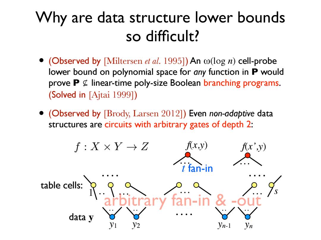
Why are data structure lower bounds so difficult? (Observed by Miltersen et al.1995])An (log n)cell-probe lower bound on polynomial space for any function in P would prove P g linear-time poly-size Boolean branching programs. (Solved in [Ajtai 1999]) (Observed by Brody,Larsen 2012])Even non-adaptive data structures are circuits with arbitrary gates of depth 2: f:XxY→Z fx,y) A,y) ifan-in data y y2 yn-1 n
Why are data structure lower bounds so difficult? • (Observed by [Miltersen et al. 1995]) An ω(log n) cell-probe lower bound on polynomial space for any function in P would prove P ⊈ linear-time poly-size Boolean branching programs. (Solved in [Ajtai 1999]) • (Observed by [Brody, Larsen 2012]) Even non-adaptive data structures are circuits with arbitrary gates of depth 2: f : X ⇥ Y ! Z data y y1 y2 yn-1 yn table cells: f(x,y) f(x’,y) arbitrary fan-in & -out t fan-in 1 s
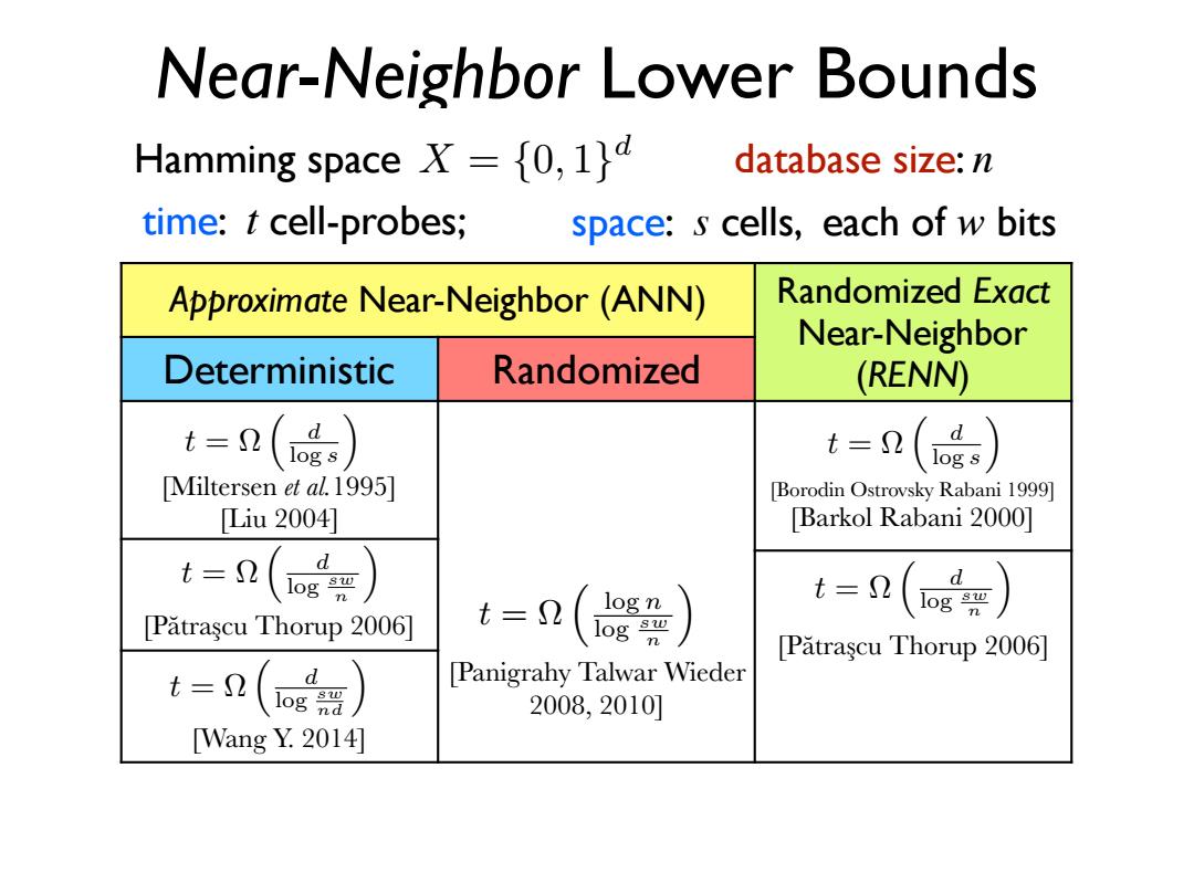
Near-Neighbor Lower Bounds Hamming space={0,1)d database size:n time:t cell-probes; space:s cells,each of w bits Approximate Near-Neighbor(ANN) Randomized Exact Near-Neighbor Deterministic Randomized (RENN) t=2 d log s t=2 () [Miltersen et al.1995] Borodin Ostrovsky Rabani 1999] Liu2004] [Barkol Rabani 2000] t=2( d log logn t=(e袋) Patrascu Thorup 2006] t=( Patrascu Thorup 2006] t=n() Panigrahy Talwar Wieder 2008,2010] [Wang Y.2014]
database size: n Approximate Near-Neighbor (ANN) Randomized Exact Near-Neighbor Deterministic Randomized (RENN) Near-Neighbor Lower Bounds Hamming space X = {0, 1}d time: t cell-probes; space: s cells, each of w bits t = ⌦ ⇣ d log s ⌘ [Miltersen et al.1995] [Liu 2004] t = ⌦ ⇣ d log sw n ⌘ [Pătraşcu Thorup 2006] t = ⌦ ⇣ d log sw nd ⌘ [Wang Y. 2014] t = ⌦ ⇣ log n log sw n ⌘ [Panigrahy Talwar Wieder 2008, 2010] t = ⌦ ⇣ d log sw n ⌘ [Pătraşcu Thorup 2006] t = ⌦ ⇣ d log s ⌘ [Borodin Ostrovsky Rabani 1999] [Barkol Rabani 2000]