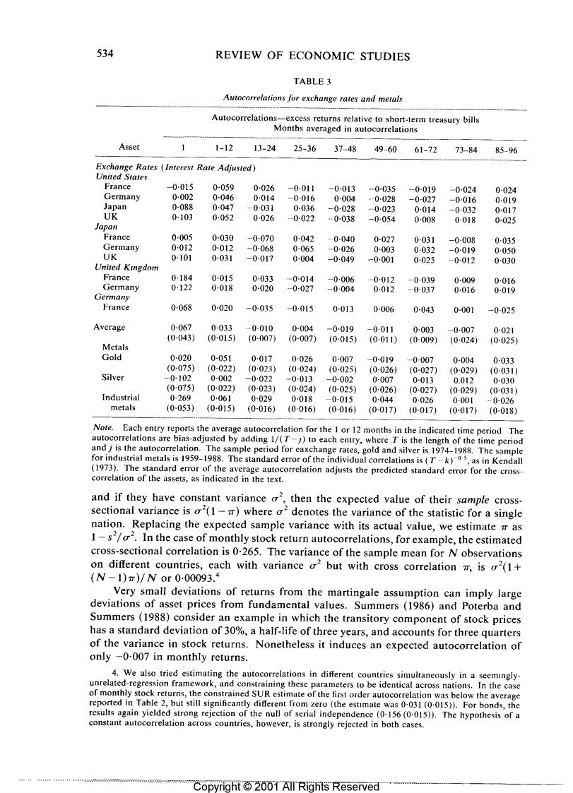
534 REVIEW OF ECONOMIC STUDIES TABLE 3 Autocorrelations for exchange rates and metals Autocorrelations-excess returns relative to short-term treasury bills Months averaged in autocorrelations Asset 1-12 13-24 25-36 37-48 49-60 61-72 73-84 85-96 Exchange Rates (Interest Rate Adjusted) United States France -0-015 0-059 0-026 -0011 -0-013 -0-035 -0-019 0-024 0-024 Germany 0-002 0046 0-014 -0016 0-004 -0028 -0027 -0-016 0-019 Japan 0-088 0047 -0-031 0-036 -0028 -0023 0014 -0-032 0017 UK 0-103 0052 0-026 -0-022 …0038 -0054 0-008 0-018 0-025 Japan France 0-005 0-030 -0-070 0-042 -0-040 0-027 0031 -0-008 0035 Germany 0-012 0-012 -0-068 0-065 -0-026 0-003 0-032 -0-019 0050 UK 0-101 0-031 -0-017 0-004 -0-049 -0-001 0025 -0012 0-030 United Kingdom France 0-184 0015 0-033 -0-014 -0-006 -0012 -0039 0009 0-016 Germany 0-122 0018 0-020 -0-027 -0-004 0-012 -0-037 0016 0-019 Germany France 0-068 0-020 -0-035 -0015 0013 0-006 0-043 0-001 -0-025 Average 0-067 0·033 -0-010 0-004 -0019 -0011 0-003 -0-007 0021 (0-043) (0-015) (0-007) (0007) (0-015) (0-011) (0-009) (0024) (0-025) Metals Gold 0-020 0-051 0017 0026 0-007 -0-019 -0-007 0-004 0-033 (0075 (0-022) (0-023 (0-024) (0-025) (0-026) (0-027) (0-029) (0-0311 Silver -0-102 0-002 -0-022 -0-013 -0002 0-007 0-013 0.012 0-030 (0-075 (0022) (0-023) (0024) (0025) (0-026) (0027) (0029) (0-031) Industrial 0269 0061 0-029 0-018 -0015 0044 0-026 0001 -0-026 metals (0-053) (0-015) (0-016) (0016) (0016) (0-017)0-0171 (0017) (0-018) Note.Each entry reports the average autocorrelation for the 1 or 12 months in the indicated time period The autocorrelations are bias-adjusted by adding 1/(T-J)to each entry,where T is the length of the time period and j is the autocorrelation.The sample period for eaxchange rates,gold and silver is 1974-1988.The sample for industrial metals is 1959-1988.The standard error of the individual correlations is (Tk),as in Kendall (1973).The standard error of the average autocorrelation adjusts the predicted standard error for the cross- correlation of the assets,as indicated in the text. and if they have constant variance o",then the expected value of their sample cross- sectional variance is o2(1)where o2denotes the variance of the statistic for a single nation.Replacing the expected sample variance with its actual value,we estimate m as 1-s2/o2.In the case of monthly stock return autocorrelations,for example,the estimated cross-sectional correlation is 0.265.The variance of the sample mean for N observations on different countries,each with variance o2 but with cross correlation m,is (1+ (N-1)π)/Nor000093.4 Very small deviations of returns from the martingale assumption can imply large deviations of asset prices from fundamental values.Summers (1986)and Poterba and Summers (1988)consider an example in which the transitory component of stock prices has a standard deviation of 30%,a half-life of three years,and accounts for three quarters of the variance in stock returns.Nonetheless it induces an expected autocorrelation of only -0-007 in monthly returns. 4.We also tried estimating the autocorrelations in different countries simultaneously in a seemingly- unrelated-regression framework,and constraining these parameters to be identical across nations.In the case of monthly stock returns,the constrained SUR estimate of the first order autocorrelation was below the average reported in Table 2,but still significantly different from zero (the estimate was 0-031(0-015)).For bonds,the results again yielded strong rejection of the null of serial independence (0-156(0-015)).The hypothesis of a constant autocorrelation across countries,however,is strongly rejected in both cases. Copyright 2001 All Rights Reserved
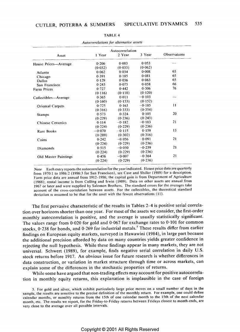
CUTLER,POTERBA SUMMERS SPECULATIVE DYNAMICS 535 TABLE 4 Autocorrelations for alternatice assets Autocorrelation Asset 1 Year 2 Year 3 Year Observations House Prices-Average 0-206 0-083 0053 (0-032) (0033) (0-062) Atlanta 0-062 0034 0-008 65 Chicago 0391 0-185 0-081 65 Dallas 0-129 0-036 0-063 65 San Francisco 0243 0-075 0-058 66 Farm Prices 0-727 0-442 0-306 76 (0-116) (0-118) (0120) Collectibles--Average 0-365 0011 -0-103 (0-160) (0-153) (0-152) Oriental Carpets 0725 0-163 -0-105 11 (0-316) (0333) (0-354) Stamps 0573 0-324 0-105 20 (0229j (0-236) (0-243) Chinese Ceramics 0114 -0-182 -0183 (0224) (0229) (0-236) Rare Books -0-070 0-115 0159 13 (0289) (0302) (0-316) Coins 0-242 -0056 0-091 21 (0-224) (0·229) (0236) Diamonds 0-515 -0-050 -0-239 21 (0224) (0229) (0-236) Old Master Paintings 0456 -0-007 -0364 21 (0:224) (0-229) (0236) Note Each entry reports the autocorrelation for the year indicated.House price data are quarterly from 1970:1 to 1986:2 (1986:3 for San Francisco),see Case and Shiller (1989)for a description. Farm price data are annual from 1912-1986;the capital gain is from Department of Agriculture (1988);rental income is from Colling and Irwin (1989).Data on other assets are annual from 1967 or later and were supplied by Salomon Brothers.The standard errors for the averages take account of the cross-correlation between assets.For the collectibles,the theoretical standard deviation is assumed to be that for the asset with the fewest observations (11). The first pervasive characteristic of the results in Tables 2-4 is positive serial correla- tion over horizons shorter than one year.For most of the assets we consider,the first-order monthly autocorrelation is positive,and the average is usually statistically significant. The values range from 0-020 for gold and 0.067 for exchange rates to 0.101 for common stocks,0.238 for bonds,and 0.269 for industrial metals.These results differ from earlier findings on European equity markets,surveyed in Hawawini(1984),in large part because the additional precision afforded by data on many countries yields greater confidence in rejecting the null hypothesis.While these findings appear in many markets,they are not universal.Schwert (1989),for example,finds negative serial correlation in daily U.S. stock returns before 1917.An obvious issue for future research is whether differences in data construction,or variation in market structure through time or across markets,can explain some of the differences in the stochastic properties of returns. While some have argued that non-trading effects may account for positive autocorrela- tion in monthly equity returns,this explanation is implausible in the case of foreign 5.For gold and silver,which exhibit particularly large price moves on a small number of days in the sample,the results are sensitive to the precise definition of the monthly return.For example,one could define calendar months,or monthly returns from the 15th of one calendar month to the 15th of the next calendar month,etc.The results we report,for the Friday-to-Friday returns between Fridays closest to month-ends,are very close to the average over all possible intervals. Copyright 2001 All Rights Reserved