136 BURGES ● 0 @ -b w 0 ●】 Figure 6.Linear separating hyperplanes for the non-separable case where the ui are the Lagrange multipliers introduced to enforce positivity of the The KKT conditions for the primal problem are therefore(note i runs from I to the number of training points,and from I to the dimension of the data) aLP OWv =w-∑aw=0 (48) 0=-∑a%=0 (49) OLP 0c: =C-ai-4=0 (50) (x·w+b)-1+ξ≥0 (51) 5.≥0 (52) a1≥0 (53) 4≥0 (54) a:{(xi·w+b)-1+E}=0 (55) h5=0 (56) As before,we can use the KKT complementarity conditions,Egs.(55)and(56),to determine the threshold b.Note that Eq.(50)combined with Eq.(56)shows that =0if i<C.Thus we can simply take any training point for which0<a<Cto use Eq.(55) (with i=0)to compute b.(As before,it is numerically wiser to take the average over all such training points.) 3.6.A Mechanical Analogy Consider the case in which the data are in R2.Suppose that the i'th support vector exerts a force Fi=yw on a stiff sheet lying along the decision surface(the"decision sheet")
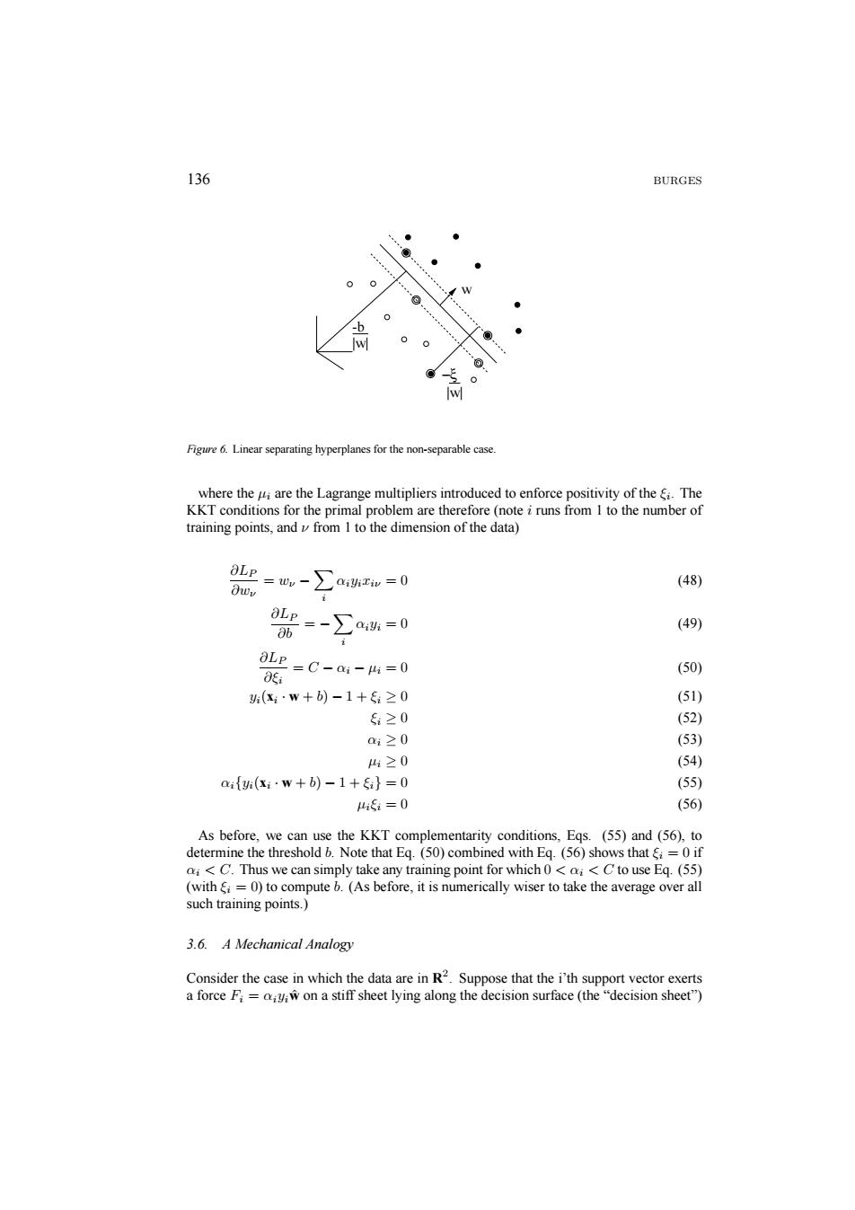
136 BURGES -b −ξ |w| |w| w Figure 6. Linear separating hyperplanes for the non-separable case. where the µi are the Lagrange multipliers introduced to enforce positivity of the ξi. The KKT conditions for the primal problem are therefore (note i runs from 1 to the number of training points, and ν from 1 to the dimension of the data) ∂LP ∂wν = wν −X i αiyixiν = 0 (48) ∂LP ∂b = − X i αiyi = 0 (49) ∂LP ∂ξi = C − αi − µi = 0 (50) yi(xi · w + b) − 1 + ξi ≥ 0 (51) ξi ≥ 0 (52) αi ≥ 0 (53) µi ≥ 0 (54) αi{yi(xi · w + b) − 1 + ξi} = 0 (55) µiξi = 0 (56) As before, we can use the KKT complementarity conditions, Eqs. (55) and (56), to determine the threshold b. Note that Eq. (50) combined with Eq. (56) shows that ξi = 0 if αi < C. Thus we can simply take any training point for which 0 < αi < C to use Eq. (55) (with ξi = 0) to compute b. (As before, it is numerically wiser to take the average over all such training points.) 3.6. A Mechanical Analogy Consider the case in which the data are in R2. Suppose that the i’th support vector exerts a force Fi = αiyiwˆ on a stiff sheet lying along the decision surface (the “decision sheet”)
SUPPORT VECTOR MACHINES 137 Figure 7.The linear case,separable(left)and not(right).The background colour shows the shape of the decision surface. (here w denotes the unit vector in the direction w).Then the solution (46)satisfies the conditions of mechanical equilibrium: ∑Forces=∑a,gm=0 (57) ∑Torques=∑A(a,)=WAW=0. (58) (Here the si are the support vectors,and A denotes the vector product.)For data in R", clearly the condition that the sum of forces vanish is still met.One can easily show that the torque also vanishes.9 This mechanical analogy depends only on the form of the solution (46).and therefore holds for both the separable and the non-separable cases.In fact this analogy holds in general(ie.,also for the nonlinear case described below).The analogy emphasizes the interesting point that the"most important"data points are the support vectors with highest values of a,since they exert the highest forces on the decision sheet.For the non-separable case,the upper bound ai<C corresponds to an upper bound on the force any given point is allowed to exert on the sheet.This analogy also provides a reason(as good as any other) to call these particular vectors"support vectors 3.7.Examples by Pictures Figure 7 shows two examples of a two-class pattern recognition problem,one separable and one not.The two classes are denoted by circles and disks respectively.Support vectors are identified with an extra circle.The error in the non-separable case is identified with a cross.The reader is invited to use Lucent's SVM Applet (Burges,Knirsch and Haratsch. 1996)to experiment and create pictures like these(if possible,try using 16 or 24 bit color). 4.Nonlinear Support Vector Machines How can the above methods be generalized to the case where the decision function1 is not a linear function of the data?(Boser,Guyon and Vapnik,1992),showed that a rather old
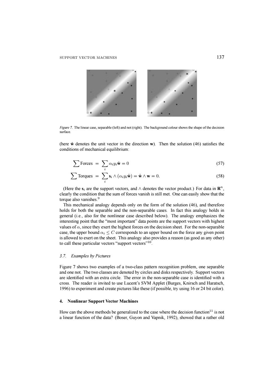
SUPPORT VECTOR MACHINES 137 Figure 7. The linear case, separable (left) and not (right). The background colour shows the shape of the decision surface. (here wˆ denotes the unit vector in the direction w). Then the solution (46) satisfies the conditions of mechanical equilibrium: XForces = X i αiyiwˆ = 0 (57) XTorques = X i si ∧ (αiyiwˆ) = wˆ ∧ w = 0. (58) (Here the si are the support vectors, and ∧ denotes the vector product.) For data in Rn, clearly the condition that the sum of forces vanish is still met. One can easily show that the torque also vanishes.9 This mechanical analogy depends only on the form of the solution (46), and therefore holds for both the separable and the non-separable cases. In fact this analogy holds in general (i.e., also for the nonlinear case described below). The analogy emphasizes the interesting point that the “most important” data points are the support vectors with highest values of α, since they exert the highest forces on the decision sheet. For the non-separable case, the upper bound αi ≤ C corresponds to an upper bound on the force any given point is allowed to exert on the sheet. This analogy also provides a reason (as good as any other) to call these particular vectors “support vectors”10. 3.7. Examples by Pictures Figure 7 shows two examples of a two-class pattern recognition problem, one separable and one not. The two classes are denoted by circles and disks respectively. Support vectors are identified with an extra circle. The error in the non-separable case is identified with a cross. The reader is invited to use Lucent’s SVM Applet (Burges, Knirsch and Haratsch, 1996) to experiment and create pictures like these (if possible, try using 16 or 24 bit color). 4. Nonlinear Support Vector Machines How can the above methods be generalized to the case where the decision function11 is not a linear function of the data? (Boser, Guyon and Vapnik, 1992), showed that a rather old