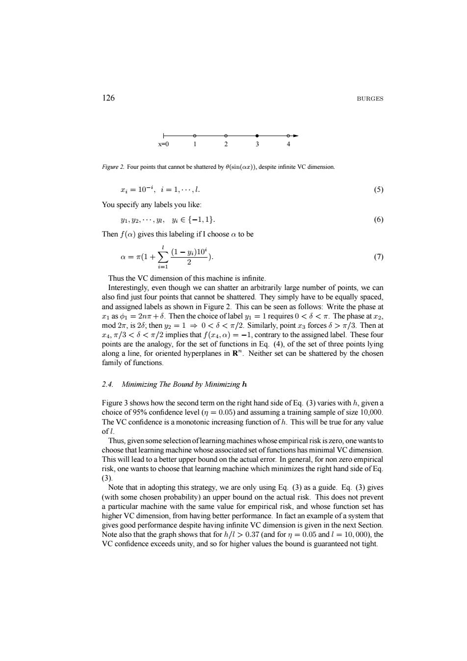
126 BURGES 人 x=0 1 2 Figure 2.Four points that cannot be shattered by 0(sin()),despite infinite VC dimension x1=10-i,i=1,…,l. (5) You specify any labels you like 1,2,…,,∈{-1,1} (6) Then f(a)gives this labeling if I choose a to be a=π1+∑-h10 (7) 2 Thus the VC dimension of this machine is infinite. Interestingly,even though we can shatter an arbitrarily large number of points,we can also find just four points that cannot be shattered.They simply have to be equally spaced, and assigned labels as shown in Figure 2.This can be seen as follows:Write the phase at xI as o1=2nm+0.Then the choice of label y =1 requires 0<o<T.The phase at x2. mod 2n,is 26;then y2 =10<6</2.Similarly,point z3 forces 6>/3.Then at x4,/3<6<T/2 implies that f(x4,a)=-1,contrary to the assigned label.These four points are the analogy,for the set of functions in Eq.(4),of the set of three points lying along a line,for oriented hyperplanes in R".Neither set can be shattered by the chosen family of functions. 2.4.Minimizing The Bound by Minimizing h Figure 3 shows how the second term on the right hand side of Eq.(3)varies with h,given a choice of 95%confidence level (n=0.05)and assuming a training sample of size 10,000. The VC confidence is a monotonic increasing function of h.This will be true for any value of l. Thus,given some selection oflearning machines whose empirical risk is zero,one wants to choose that learning machine whose associated set of functions has minimal VC dimension. This will lead to a better upper bound on the actual error.In general,for non zero empirical risk,one wants to choose that learning machine which minimizes the right hand side of Eq. (3) Note that in adopting this strategy,we are only using Eq.(3)as a guide.Eq.(3)gives (with some chosen probability)an upper bound on the actual risk.This does not prevent a particular machine with the same value for empirical risk,and whose function set has higher VC dimension,from having better performance.In fact an example of a system that gives good performance despite having infinite VC dimension is given in the next Section. Note also that the graph shows that for h/>0.37 (and for n =0.05 and l 10,000),the VC confidence exceeds unity,and so for higher values the bound is guaranteed not tight
126 BURGES x=0 1234 Figure 2. Four points that cannot be shattered by θ(sin(αx)), despite infinite VC dimension. xi = 10−i , i = 1, ··· ,l. (5) You specify any labels you like: y1, y2, ··· , yl, yi ∈ {−1, 1}. (6) Then f(α) gives this labeling if I choose α to be α = π(1 +X l i=1 (1 − yi)10i 2 ). (7) Thus the VC dimension of this machine is infinite. Interestingly, even though we can shatter an arbitrarily large number of points, we can also find just four points that cannot be shattered. They simply have to be equally spaced, and assigned labels as shown in Figure 2. This can be seen as follows: Write the phase at x1 as φ1 = 2nπ +δ. Then the choice of label y1 = 1 requires 0 <δ<π. The phase at x2, mod 2π, is 2δ; then y2 = 1 ⇒ 0 < δ < π/2. Similarly, point x3 forces δ > π/3. Then at x4, π/3 < δ < π/2 implies that f(x4, α) = −1, contrary to the assigned label. These four points are the analogy, for the set of functions in Eq. (4), of the set of three points lying along a line, for oriented hyperplanes in Rn. Neither set can be shattered by the chosen family of functions. 2.4. Minimizing The Bound by Minimizing h Figure 3 shows how the second term on the right hand side of Eq. (3) varies with h, given a choice of 95% confidence level (η = 0.05) and assuming a training sample of size 10,000. The VC confidence is a monotonic increasing function of h. This will be true for any value of l. Thus, given some selection of learning machines whose empirical risk is zero, one wants to choose that learning machine whose associated set of functions has minimal VC dimension. This will lead to a better upper bound on the actual error. In general, for non zero empirical risk, one wants to choose that learning machine which minimizes the right hand side of Eq. (3). Note that in adopting this strategy, we are only using Eq. (3) as a guide. Eq. (3) gives (with some chosen probability) an upper bound on the actual risk. This does not prevent a particular machine with the same value for empirical risk, and whose function set has higher VC dimension, from having better performance. In fact an example of a system that gives good performance despite having infinite VC dimension is given in the next Section. Note also that the graph shows that for h/l > 0.37 (and for η = 0.05 and l = 10, 000), the VC confidence exceeds unity, and so for higher values the bound is guaranteed not tight
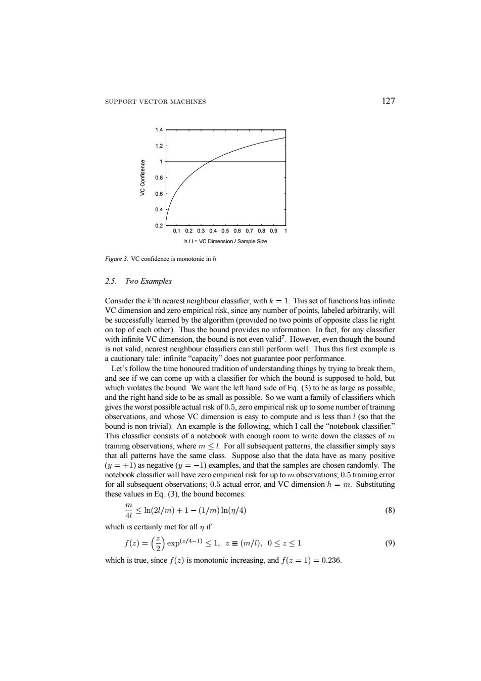
SUPPORT VECTOR MACHINES 127 1.4 1.2 0.8 9 0.6 0.4 02 0.1020.30.40.50.60.70.80.91 h/I=VC Dimension Sample Size Figure 3.VC confidence is monotonic in h 2.5.Two Examples Consider the k'th nearest neighbour classifier.with k=1.This set of functions has infinite VC dimension and zero empirical risk,since any number of points,labeled arbitrarily,will be successfully learned by the algorithm(provided no two points of opposite class lie right on top of each other).Thus the bound provides no information.In fact,for any classifier with infinite VC dimension,the bound is not even valid?.However,even though the bound is not valid,nearest neighbour classifiers can still perform well.Thus this first example is a cautionary tale:infinite"capacity"does not guarantee poor performance. Let's follow the time honoured tradition of understanding things by trying to break them, and see if we can come up with a classifier for which the bound is supposed to hold,but which violates the bound.We want the left hand side of Eq.(3)to be as large as possible, and the right hand side to be as small as possible.So we want a family of classifiers which gives the worst possible actual risk of0.5,zero empirical risk up to some number of training observations,and whose VC dimension is easy to compute and is less than l(so that the bound is non trivial).An example is the following,which I call the"notebook classifier." This classifier consists of a notebook with enough room to write down the classes of m training observations,where m<1.For all subsequent patterns,the classifier simply says that all patterns have the same class.Suppose also that the data have as many positive (y=+1)as negative (y=-1)examples,and that the samples are chosen randomly.The notebook classifier will have zero empirical risk for up to m observations;0.5 training error for all subsequent observations;0.5 actual error,and VC dimension h=m.Substituting these values in Eq.(3),the bound becomes: ≤n(2/m)+1-(1/m)ln(/④ m (8) which is certainly met for all n if fa=()exp-)≤1,z=m/0,0≤z≤1 (9) which is true,since f(z)is monotonic increasing,and f(=1)=0.236
SUPPORT VECTOR MACHINES 127 0.2 0.4 0.6 0.8 1 1.2 1.4 0.1 0.2 0.3 0.4 0.5 0.6 0.7 0.8 0.9 1 VC Confidence h / l = VC Dimension / Sample Size Figure 3. VC confidence is monotonic in h 2.5. Two Examples Consider the k’th nearest neighbour classifier, with k = 1. This set of functions has infinite VC dimension and zero empirical risk, since any number of points, labeled arbitrarily, will be successfully learned by the algorithm (provided no two points of opposite class lie right on top of each other). Thus the bound provides no information. In fact, for any classifier with infinite VC dimension, the bound is not even valid7. However, even though the bound is not valid, nearest neighbour classifiers can still perform well. Thus this first example is a cautionary tale: infinite “capacity” does not guarantee poor performance. Let’s follow the time honoured tradition of understanding things by trying to break them, and see if we can come up with a classifier for which the bound is supposed to hold, but which violates the bound. We want the left hand side of Eq. (3) to be as large as possible, and the right hand side to be as small as possible. So we want a family of classifiers which gives the worst possible actual risk of 0.5, zero empirical risk up to some number of training observations, and whose VC dimension is easy to compute and is less than l (so that the bound is non trivial). An example is the following, which I call the “notebook classifier.” This classifier consists of a notebook with enough room to write down the classes of m training observations, where m ≤ l. For all subsequent patterns, the classifier simply says that all patterns have the same class. Suppose also that the data have as many positive (y = +1) as negative (y = −1) examples, and that the samples are chosen randomly. The notebook classifier will have zero empirical risk for up to m observations; 0.5 training error for all subsequent observations; 0.5 actual error, and VC dimension h = m. Substituting these values in Eq. (3), the bound becomes: m 4l ≤ ln(2l/m)+1 − (1/m) ln(η/4) (8) which is certainly met for all η if f(z) = ³z 2 ´ exp(z/4−1) ≤ 1, z ≡ (m/l), 0 ≤ z ≤ 1 (9) which is true, since f(z) is monotonic increasing, and f(z = 1) = 0.236
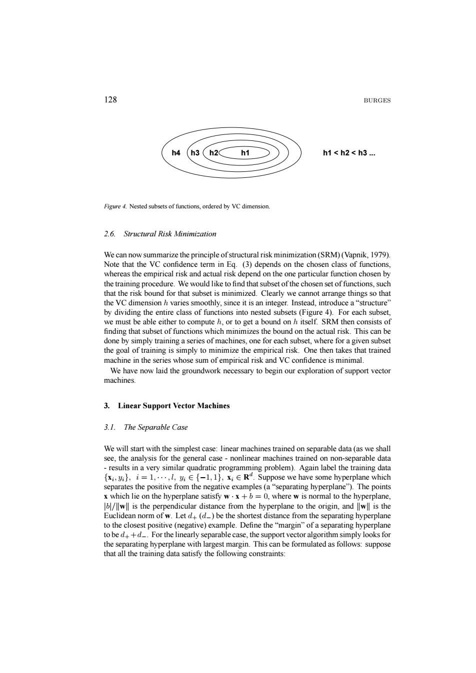
128 BURGES h4 (h3(h2h1 h1<h2<h3 Figure 4.Nested subsets of functions,ordered by VC dimension 2.6.Structural Risk Minimization We can now summarize the principle of structural risk minimization(SRM)(Vapnik,1979). Note that the VC confidence term in Eq.(3)depends on the chosen class of functions, whereas the empirical risk and actual risk depend on the one particular function chosen by the training procedure.We would like to find that subset of the chosen set of functions,such that the risk bound for that subset is minimized.Clearly we cannot arrange things so that the VC dimension h varies smoothly,since it is an integer.Instead,introduce a"structure" by dividing the entire class of functions into nested subsets(Figure 4).For each subset we must be able either to compute h,or to get a bound on h itself.SRM then consists of finding that subset of functions which minimizes the bound on the actual risk.This can be done by simply training a series of machines,one for each subset,where for a given subset the goal of training is simply to minimize the empirical risk.One then takes that trained machine in the series whose sum of empirical risk and VC confidence is minimal. We have now laid the groundwork necessary to begin our exploration of support vector machines. 3.Linear Support Vector Machines 3.1.The Separable Case We will start with the simplest case:linear machines trained on separable data(as we shall see,the analysis for the general case-nonlinear machines trained on non-separable data results in a very similar quadratic programming problem).Again label the training data x,,i=1,...,l,i-1,1),xiE Rd.Suppose we have some hyperplane which separates the positive from the negative examples(a"separating hyperplane").The points x which lie on the hyperplane satisfy w.x+b=0,where w is normal to the hyperplane, wll is the perpendicular distance from the hyperplane to the origin,and lwll is the Euclidean norm of w.Let d(d)be the shortest distance from the separating hyperplane to the closest positive(negative)example.Define the"margin"of a separating hyperplane to be d+d_.For the linearly separable case,the support vector algorithm simply looks for the separating hyperplane with largest margin.This can be formulated as follows:suppose that all the training data satisfy the following constraints:
128 BURGES h4 h1 < h2 < h3 ... h3 h2 h1 Figure 4. Nested subsets of functions, ordered by VC dimension. 2.6. Structural Risk Minimization We can now summarize the principle of structural risk minimization (SRM) (Vapnik, 1979). Note that the VC confidence term in Eq. (3) depends on the chosen class of functions, whereas the empirical risk and actual risk depend on the one particular function chosen by the training procedure. We would like to find that subset of the chosen set of functions, such that the risk bound for that subset is minimized. Clearly we cannot arrange things so that the VC dimension h varies smoothly, since it is an integer. Instead, introduce a “structure” by dividing the entire class of functions into nested subsets (Figure 4). For each subset, we must be able either to compute h, or to get a bound on h itself. SRM then consists of finding that subset of functions which minimizes the bound on the actual risk. This can be done by simply training a series of machines, one for each subset, where for a given subset the goal of training is simply to minimize the empirical risk. One then takes that trained machine in the series whose sum of empirical risk and VC confidence is minimal. We have now laid the groundwork necessary to begin our exploration of support vector machines. 3. Linear Support Vector Machines 3.1. The Separable Case We will start with the simplest case: linear machines trained on separable data (as we shall see, the analysis for the general case - nonlinear machines trained on non-separable data - results in a very similar quadratic programming problem). Again label the training data {xi, yi}, i = 1, ··· ,l, yi ∈ {−1, 1}, xi ∈ Rd. Suppose we have some hyperplane which separates the positive from the negative examples (a “separating hyperplane”). The points x which lie on the hyperplane satisfy w · x + b = 0, where w is normal to the hyperplane, |b|/kwk is the perpendicular distance from the hyperplane to the origin, and kwk is the Euclidean norm of w. Let d+ (d−) be the shortest distance from the separating hyperplane to the closest positive (negative) example. Define the “margin” of a separating hyperplane to be d+ +d−. For the linearly separable case, the support vector algorithm simply looks for the separating hyperplane with largest margin. This can be formulated as follows: suppose that all the training data satisfy the following constraints:
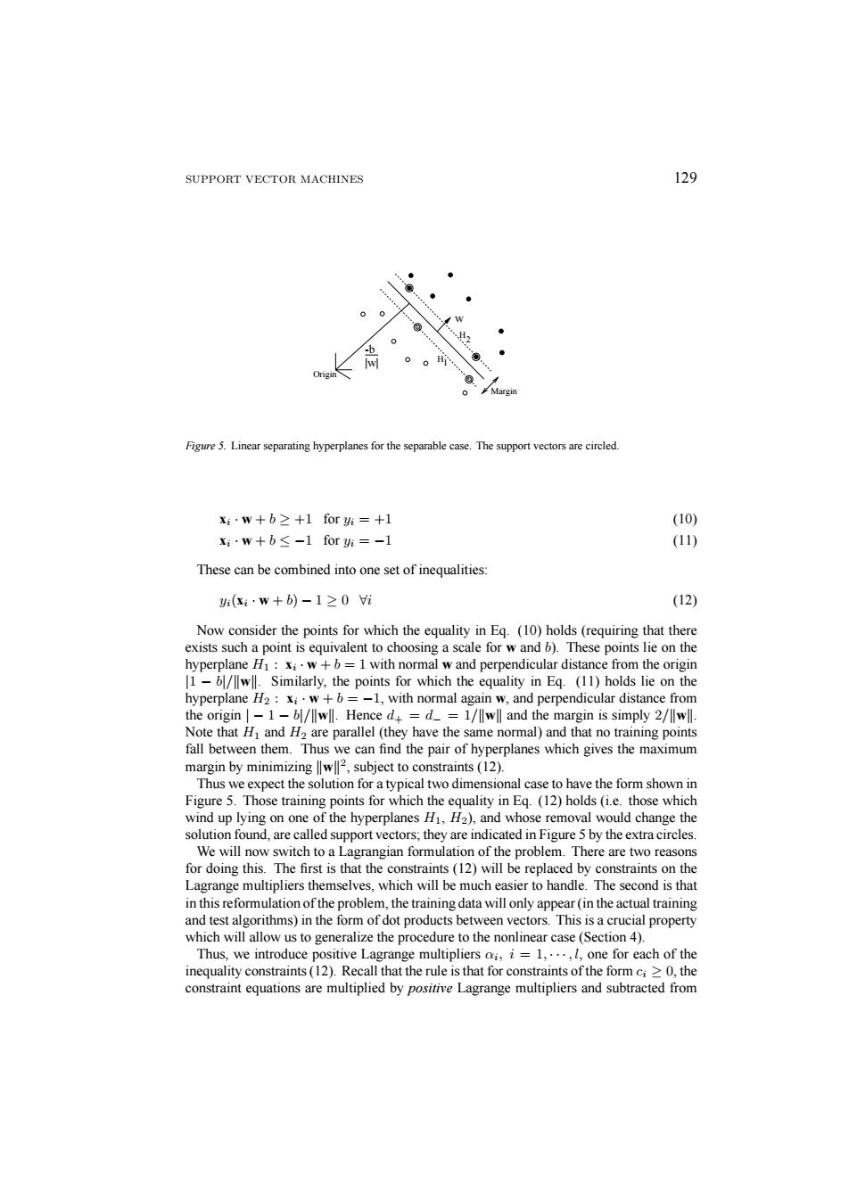
SUPPORT VECTOR MACHINES 129 ● H @ Margin Figure 5.Linear separating hyperplanes for the separable case.The support vectors are circled. x:·w+b≥+1for=+1 (10) x;·w+b≤-1fori=-1 (11) These can be combined into one set of inequalities: (x·w+b)-1≥0i (12) Now consider the points for which the equality in Eq.(10)holds(requiring that there exists such a point is equivalent to choosing a scale for w and b).These points lie on the hyperplane H1:xi.w+6=1 with normal w and perpendicular distance from the origin 1-b/wll.Similarly,the points for which the equality in Eq.(11)holds lie on the hyperplane H2:xiw+b=-1,with normal again w,and perpendicular distance from the origin-1-bl/llwll.Hence d=d=1/wll and the margin is simply 2/wll. Note that Hi and H2 are parallel(they have the same normal)and that no training points fall between them.Thus we can find the pair of hyperplanes which gives the maximum margin by minimizing w2,subject to constraints(12). Thus we expect the solution for a typical two dimensional case to have the form shown in Figure 5.Those training points for which the equality in Eq.(12)holds(i.e.those which wind up lying on one of the hyperplanes H1,H2),and whose removal would change the solution found,are called support vectors;they are indicated in Figure 5 by the extra circles. We will now switch to a Lagrangian formulation of the problem.There are two reasons for doing this.The first is that the constraints(12)will be replaced by constraints on the Lagrange multipliers themselves,which will be much easier to handle.The second is that in this reformulation of the problem,the training data will only appear(in the actual training and test algorithms)in the form of dot products between vectors.This is a crucial property which will allow us to generalize the procedure to the nonlinear case(Section 4). Thus,we introduce positive Lagrange multipliers o,i=1,...,l,one for each of the inequality constraints(12).Recall that the rule is that for constraints of the form ci>0,the constraint equations are multiplied by positive Lagrange multipliers and subtracted from
SUPPORT VECTOR MACHINES 129 -b |w| w Origin Margin H1 H2 Figure 5. Linear separating hyperplanes for the separable case. The support vectors are circled. xi · w + b ≥ +1 for yi = +1 (10) xi · w + b ≤ −1 for yi = −1 (11) These can be combined into one set of inequalities: yi(xi · w + b) − 1 ≥ 0 ∀i (12) Now consider the points for which the equality in Eq. (10) holds (requiring that there exists such a point is equivalent to choosing a scale for w and b). These points lie on the hyperplane H1 : xi · w + b = 1 with normal w and perpendicular distance from the origin |1 − b|/kwk. Similarly, the points for which the equality in Eq. (11) holds lie on the hyperplane H2 : xi · w + b = −1, with normal again w, and perpendicular distance from the origin | − 1 − b|/kwk. Hence d+ = d− = 1/kwk and the margin is simply 2/kwk. Note that H1 and H2 are parallel (they have the same normal) and that no training points fall between them. Thus we can find the pair of hyperplanes which gives the maximum margin by minimizing kwk2, subject to constraints (12). Thus we expect the solution for a typical two dimensional case to have the form shown in Figure 5. Those training points for which the equality in Eq. (12) holds (i.e. those which wind up lying on one of the hyperplanes H1, H2), and whose removal would change the solution found, are called support vectors; they are indicated in Figure 5 by the extra circles. We will now switch to a Lagrangian formulation of the problem. There are two reasons for doing this. The first is that the constraints (12) will be replaced by constraints on the Lagrange multipliers themselves, which will be much easier to handle. The second is that in this reformulation of the problem, the training data will only appear (in the actual training and test algorithms) in the form of dot products between vectors. This is a crucial property which will allow us to generalize the procedure to the nonlinear case (Section 4). Thus, we introduce positive Lagrange multipliers αi, i = 1, ··· , l, one for each of the inequality constraints (12). Recall that the rule is that for constraints of the form ci ≥ 0, the constraint equations are multiplied by positive Lagrange multipliers and subtracted from
130 BURGES the objective function,to form the Lagrangian.For equality constraints,the Lagrange multipliers are unconstrained.This gives Lagrangian: Lp三w2-∑a(w+b)+∑a4 (13) 1=1 i=1 We must now minimize Lp with respect to w,b,and simultaneously require that the derivatives of Lp with respect to all the ai vanish,all subject to the constraints ai>0 (let's call this particular set of constraints C1).Now this is a convex quadratic programming problem,since the objective function is itself convex,and those points which satisfy the constraints also form a convex set (any linear constraint defines a convex set,and a set of N simultaneous linear constraints defines the intersection of N convex sets,which is also a convex set).This means that we can equivalently solve the following"dual"problem: maximize Lp,subject to the constraints that the gradient of Lp with respect to w and b vanish,and subject also to the constraints that the a;>0(let's call that particular set of constraints C2).This particular dual formulation of the problem is called the Wolfe dual (Fletcher,1987).It has the property that the maximum of Lp,subject to constraints C2, occurs at the same values of the w,b and a,as the minimum of Lp,subject to constraints C18 Requiring that the gradient of Lp with respect to w and b vanish give the conditions: w=∑a (14) ∑班=0, (15) Since these are equality constraints in the dual formulation,we can substitute them into Eq.(13)to give n=∑a-∑aw (16) 1.3 Note that we have now given the Lagrangian different labels(P for primal,D for dual)to emphasize that the two formulations are different:Lp and Lp arise from the same objective function but with different constraints:and the solution is found by minimizing Lp or by maximizing Lp.Note also that if we formulate the problem with 6 =0,which amounts to requiring that all hyperplanes contain the origin,the constraint(15)does not appear.This is a mild restriction for high dimensional spaces,since it amounts to reducing the number of degrees of freedom by one. Support vector training(for the separable,linear case)therefore amounts to maximizing Lp with respect to the subject to constraints(15)and positivity of the with solution given by (14).Notice that there is a Lagrange multiplier o for every training point.In the solution,those points for which0 are called"support vectors",and lie on one of the hyperplanes H1,H2.All other training points have o=0 and lie either on Hi or H2(such that the equality in Eq.(12)holds),or on that side of H or H2 such that the
130 BURGES the objective function, to form the Lagrangian. For equality constraints, the Lagrange multipliers are unconstrained. This gives Lagrangian: LP ≡ 1 2 kwk2 −X l i=1 αiyi(xi · w + b) +X l i=1 αi (13) We must now minimize LP with respect to w, b, and simultaneously require that the derivatives of LP with respect to all the αi vanish, all subject to the constraints αi ≥ 0 (let’s call this particular set of constraints C1). Now this is a convex quadratic programming problem, since the objective function is itself convex, and those points which satisfy the constraints also form a convex set (any linear constraint defines a convex set, and a set of N simultaneous linear constraints defines the intersection of N convex sets, which is also a convex set). This means that we can equivalently solve the following “dual” problem: maximize LP , subject to the constraints that the gradient of LP with respect to w and b vanish, and subject also to the constraints that the αi ≥ 0 (let’s call that particular set of constraints C2). This particular dual formulation of the problem is called the Wolfe dual (Fletcher, 1987). It has the property that the maximum of LP , subject to constraints C2, occurs at the same values of the w, b and α, as the minimum of LP , subject to constraints C1 8. Requiring that the gradient of LP with respect to w and b vanish give the conditions: w = X i αiyixi (14) X i αiyi = 0. (15) Since these are equality constraints in the dual formulation, we can substitute them into Eq. (13) to give LD = X i αi − 1 2 X i,j αiαjyiyjxi · xj (16) Note that we have now given the Lagrangian different labels (P for primal, D for dual) to emphasize that the two formulations are different: LP and LD arise from the same objective function but with different constraints; and the solution is found by minimizing LP or by maximizing LD. Note also that if we formulate the problem with b = 0, which amounts to requiring that all hyperplanes contain the origin, the constraint (15) does not appear. This is a mild restriction for high dimensional spaces, since it amounts to reducing the number of degrees of freedom by one. Support vector training (for the separable, linear case) therefore amounts to maximizing LD with respect to the αi, subject to constraints (15) and positivity of the αi, with solution given by (14). Notice that there is a Lagrange multiplier αi for every training point. In the solution, those points for which αi > 0 are called “support vectors”, and lie on one of the hyperplanes H1, H2. All other training points have αi = 0 and lie either on H1 or H2 (such that the equality in Eq. (12) holds), or on that side of H1 or H2 such that the