weight on the connection between the bias in layer 1 and the second node in layer 2 is given by bz() Remember,these values-wi()and b-all need to be calculated in the training phase of the ANN. Finally,the node output notation is h,wherejdenotes the node number in layer I of the network.As can be observed in the three layer network above,the output of node 2 in layer 2 has the notation of h2(2). Now that we have the notation all sorted out,it is now time to look at how you calculate the output of the network when the input and the weights are known.The process of calculating the output of the neural network given these values is called the feed-forward pass or process. 1.3 THE FEED-FORWARD PASS To demonstrate how to calculate the output from the input in neural networks,let's start with the specific case of the three layer neural network that was presented above.Below it is presented in equation form,then it will be demonstrated with a concrete example and some Python code: h② =f0w0x1+w9x2+w8x3+b) h2) =f(w+w2x2+wx3+b) he) =f(wsx+wx2+wsxa+bs) hwb(x)=h)=f(wh)+w2h2)+wh)+b) In the equation above f()refers to the node activation function,in this case the sigmoid function.The first line,)is the output of the first node in the second layer,and its inputs arewand These inputs can be traced in the three-layer connection diagram above.They are simply summed and then passed through the activation function to calculate the output of the first node.Likewise,for the other two nodes in the second layer. The final line is the output of the only node in the third and final layer,which is ultimate output of the neural network.As can be observed,rather than taking the weighted input variables(x1,x2,x3),the final node takes as input the weighted output of the nodes of the second layer(h,,),plus the weighted bias.Therefore,you can see in equation form the hierarchical nature of artificial neural networks. PAGE 10
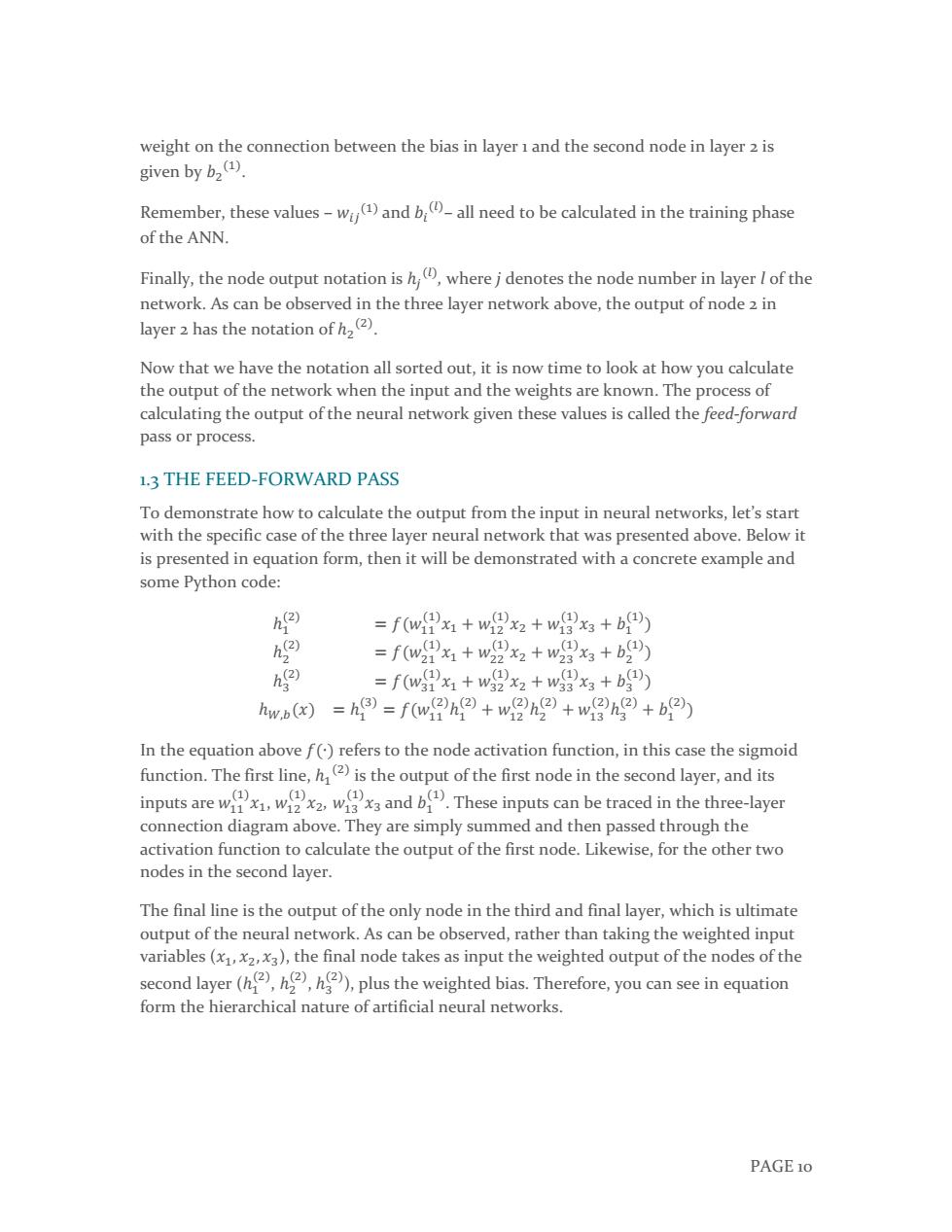
PAGE 10 weight on the connection between the bias in layer 1 and the second node in layer 2 is given by 𝑏2 (1) . Remember, these values – 𝑤𝑖𝑗 (1) and 𝑏𝑖 (𝑙) – all need to be calculated in the training phase of the ANN. Finally, the node output notation is ℎ𝑗 (𝑙) , where j denotes the node number in layer l of the network. As can be observed in the three layer network above, the output of node 2 in layer 2 has the notation of ℎ2 (2) . Now that we have the notation all sorted out, it is now time to look at how you calculate the output of the network when the input and the weights are known. The process of calculating the output of the neural network given these values is called the feed-forward pass or process. 1.3 THE FEED-FORWARD PASS To demonstrate how to calculate the output from the input in neural networks, let’s start with the specific case of the three layer neural network that was presented above. Below it is presented in equation form, then it will be demonstrated with a concrete example and some Python code: ℎ1 (2) = 𝑓(𝑤11 (1) 𝑥1 + 𝑤12 (1) 𝑥2 + 𝑤13 (1) 𝑥3 + 𝑏1 (1) ) ℎ2 (2) = 𝑓(𝑤21 (1) 𝑥1 + 𝑤22 (1) 𝑥2 + 𝑤23 (1) 𝑥3 + 𝑏2 (1) ) ℎ3 (2) = 𝑓(𝑤31 (1) 𝑥1 + 𝑤32 (1) 𝑥2 + 𝑤33 (1) 𝑥3 + 𝑏3 (1) ) ℎ𝑊,𝑏(𝑥) = ℎ1 (3) = 𝑓(𝑤11 (2) ℎ1 (2) + 𝑤12 (2) ℎ2 (2) + 𝑤13 (2) ℎ3 (2) + 𝑏1 (2) ) In the equation above 𝑓(∙) refers to the node activation function, in this case the sigmoid function. The first line, ℎ1 (2) is the output of the first node in the second layer, and its inputs are 𝑤11 (1) 𝑥1, 𝑤12 (1) 𝑥2, 𝑤13 (1) 𝑥3 and 𝑏1 (1) . These inputs can be traced in the three-layer connection diagram above. They are simply summed and then passed through the activation function to calculate the output of the first node. Likewise, for the other two nodes in the second layer. The final line is the output of the only node in the third and final layer, which is ultimate output of the neural network. As can be observed, rather than taking the weighted input variables (𝑥1, 𝑥2, 𝑥3), the final node takes as input the weighted output of the nodes of the second layer (ℎ1 (2) , ℎ2 (2) , ℎ3 (2) ), plus the weighted bias. Therefore, you can see in equation form the hierarchical nature of artificial neural networks
1.3.1 A feed-forward example Now,let's do a simple first example of the output of this neural network in Python.First things first,notice that the weights between layerandwareideally suited to matrix representation (check out this link to brush up on matrices)?Observe: (1) (1) W13 w() (1) ) (1) 0 02 023 1) (1) (1) 031 W 033 import numpy as np w1=np.array([0.2,6.2,0.2],[6.4,6.4,6.4],[0.6,6.6,6.6]) If you're not sure about how numpy arrays work,check out the documentation here.Here I have just filled up the layer 1 weight array with some example weights.We can do the same for the layer 2 weight array: w)=(w ww) w2 np.zeros((1,3)) w2[o,:]=np.array([o.5,8.5,e.5]) We can also setup some dummy values in the layer 1 bias weight array/vector,and the layer 2 bias weight(which is only a single value in this neural network structure-i.e.a scalar): b1=np.array([g,8,6.8,6.8]) b2 np.array([0.2]) Finally,before we write the main program to calculate the output from the neural network,it's handy to setup a separate Python function for the activation function: def f(x): return 1 /(1 np.exp(-x)) 1.3.2 Our first attempt at a feed-forward function Below is a simple way of calculating the output of the neural network,using nested loops in python.We'll look at more efficient ways of calculating the output shortly. PAGE 11
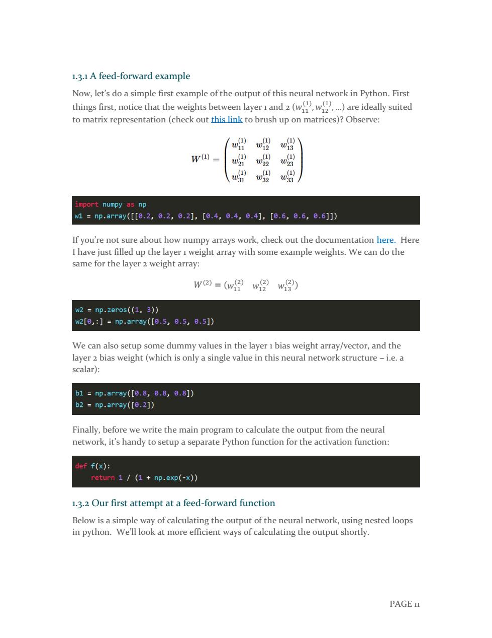
PAGE 11 1.3.1 A feed-forward example Now, let’s do a simple first example of the output of this neural network in Python. First things first, notice that the weights between layer 1 and 2 (𝑤11 (1) , 𝑤12 (1) , …) are ideally suited to matrix representation (check out this link to brush up on matrices)? Observe: If you’re not sure about how numpy arrays work, check out the documentation here. Here I have just filled up the layer 1 weight array with some example weights. We can do the same for the layer 2 weight array: 𝑊(2) = (𝑤11 (2) 𝑤12 (2) 𝑤13 (2) ) We can also setup some dummy values in the layer 1 bias weight array/vector, and the layer 2 bias weight (which is only a single value in this neural network structure – i.e. a scalar): Finally, before we write the main program to calculate the output from the neural network, it’s handy to setup a separate Python function for the activation function: 1.3.2 Our first attempt at a feed-forward function Below is a simple way of calculating the output of the neural network, using nested loops in python. We’ll look at more efficient ways of calculating the output shortly
def simple_looped_nn_calc(n_layers,x,w,b): for 1 in range(n_layers-1): #Setup the input array which the weights will be multiplied by for each layer #If it's the first layer,the input array will be the x input vector #If it's not the first layer,the input to the next layer will be the #output of the previous layer if1=0: node_in =x else: node in h #Setup the output array for the nodes in layer 1+1 h np.zeros((w[1].shape[e],)) #loop through the rows of the weight array for i in range(w[1].shape[e]): #setup the sum inside the activation function f_sum =0 #loop through the columns of the weight array for j in range(w[1].shape[1]): f_sum +w[l][i][j]node_in[j] #add the bias f_sum +b[l][i] #finally use the activation function to calculate the #i-th output i.e.h1,h2,h3 h[i]f(f_sum) return h This function takes as input the number of layers in the neural network,the x input array/vector,then Python tuples or lists of the weights and bias weights of the network, with each element in the tuple/list representing a layer I in the network.In other words, the inputs are setup in the following: W=[w1,w2] b=[b1,b2] #a dummy x input vector ×=[1,5,2.6,3.0] The function first checks what the input is to the layer of nodes/weights being considered. If we are looking at the first layer,the input to the second layer nodes is the input vector x multiplied by the relevant weights.After the first layer though,the inputs to subsequent layers are the output of the previous layers.Finally,there is a nested loop through the relevant I and j values of the weight vectors and the bias.The function uses the dimensions of the weights for each layer to figure out the number of nodes and therefore the structure of the network. PAGE 12
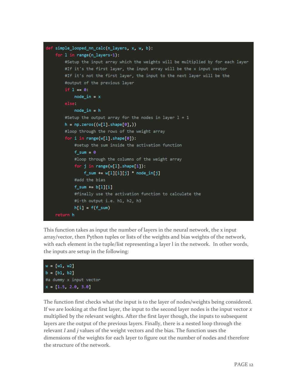
PAGE 12 This function takes as input the number of layers in the neural network, the x input array/vector, then Python tuples or lists of the weights and bias weights of the network, with each element in the tuple/list representing a layer l in the network. In other words, the inputs are setup in the following: The function first checks what the input is to the layer of nodes/weights being considered. If we are looking at the first layer, the input to the second layer nodes is the input vector x multiplied by the relevant weights. After the first layer though, the inputs to subsequent layers are the output of the previous layers. Finally, there is a nested loop through the relevant I and j values of the weight vectors and the bias. The function uses the dimensions of the weights for each layer to figure out the number of nodes and therefore the structure of the network

Calling the function: simple_looped_nn_calc(3,x,w,b) gives the output of o.8354.We can confirm this results by manually performing the calculations in the original equations: ha =f(0.2*1.5+0.2*2.0+0.2*3.0+0.8)=0.8909 ) =f(0.4*1.5+0.4*2.0+0.4*3.0+0.8)=0.9677 h92 =f(0.6*1.5+0.6*2.0+0.6*3.0+0.8)=0.9909 hw,b)=h③)=f0.5*0.8909+0.5*0.9677+0.5*0.9909+0.2)=0.8354 1.3.3 A more efficient implementation As was stated earlier-using loops isn't the most efficient way of calculating the feed forward step in Python.This is because the loops in Python are notoriously slow.An alternative,more efficient mechanism of doing the feed forward step in Python and numpy will be discussed shortly.We can benchmark how efficient the algorithm is by using the %timeit function in IPython,which runs the function a number of times and returns the average time that the function takes to run: %timeit simple_looped_nn_calc(3,x,w,b) Running this tells us that the looped feed forward takes 4ous.A result in the tens of microseconds sounds very fast,but when applied to very large practical NNs with ioos of nodes per layer,this speed will become prohibitive,especially when training the network, as will become clear later in this tutorial.If we try a four layer neural network using the same code,we get significantly worse performance-7ous in fact. 1.3.4 Vectorisation in neural networks There is a way to write the equations even more compactly,and to calculate the feed forward process in neural networks more efficiently,from a computational perspective.Firstly,we can introduce a new variablezwhich is the summated input into node I of layer I,including the bias term.So in the case of the first node in layer 2,z is equal to: 7 Wij +6四 (1) j=1 where n is the number of nodes in layer 1.Using this notation,the unwieldy previous set of equations for the example three layer network can be reduced to: PAGE13
PAGE 13 Calling the function: gives the output of 0.8354. We can confirm this results by manually performing the calculations in the original equations: ℎ1 (2) = 𝑓(0.2 ∗ 1.5 + 0.2 ∗ 2.0 + 0.2 ∗ 3.0 + 0.8) = 0.8909 ℎ2 (2) = 𝑓(0.4 ∗ 1.5 + 0.4 ∗ 2.0 + 0.4 ∗ 3.0 + 0.8) = 0.9677 ℎ3 (2) = 𝑓(0.6 ∗ 1.5 + 0.6 ∗ 2.0 + 0.6 ∗ 3.0 + 0.8) = 0.9909 ℎ𝑊,𝑏(𝑥) = ℎ1 (3) = 𝑓(0.5 ∗ 0.8909 + 0.5 ∗ 0.9677 + 0.5 ∗ 0.9909 + 0.2) = 0.8354 1.3.3 A more efficient implementation As was stated earlier – using loops isn’t the most efficient way of calculating the feed forward step in Python. This is because the loops in Python are notoriously slow. An alternative, more efficient mechanism of doing the feed forward step in Python and numpy will be discussed shortly. We can benchmark how efficient the algorithm is by using the %timeit function in IPython, which runs the function a number of times and returns the average time that the function takes to run: Running this tells us that the looped feed forward takes 40μs. A result in the tens of microseconds sounds very fast, but when applied to very large practical NNs with 100s of nodes per layer, this speed will become prohibitive, especially when training the network, as will become clear later in this tutorial. If we try a four layer neural network using the same code, we get significantly worse performance – 70μs in fact. 1.3.4 Vectorisation in neural networks There is a way to write the equations even more compactly, and to calculate the feed forward process in neural networks more efficiently, from a computational perspective. Firstly, we can introduce a new variable 𝑧𝑖 (𝑙) which is the summated input into node I of layer l, including the bias term. So in the case of the first node in layer 2, z is equal to: 𝑧1 (2) = 𝑤11 (1) 𝑥1 + 𝑤12 (1) 𝑥2 + 𝑤13 (1) 𝑥3 + 𝑏1 (1) = ∑𝑤𝑖𝑗 (1) 𝑥𝑖 + 𝑏𝑖 (1) 𝑛 𝑗=1 where n is the number of nodes in layer 1. Using this notation, the unwieldy previous set of equations for the example three layer network can be reduced to: