1.0 0.8 0.6 0.4 0.2 0.0 8 -6 一4 -20 Figure 1 The sigmoid function As can be seen in the figure above,the function is"activated"i.e.it moves from o to1 when the input x is greater than a certain value.The sigmoid function isn't a step function however,the edge is"soft",and the output doesn't change instantaneously.This means that there is a derivative of the function and this is important for the training algorithm which is discussed more in Section 1.4.5 Backpropagation in depth. 1.2.2 Nodes As mentioned previously,biological neurons are connected hierarchical networks,with the outputs of some neurons being the inputs to others.We can represent these networks as connected layers of nodes.Each node takes multiple weighted inputs,applies the activation function to the summation of these inputs,and in doing so generates an output. I'll break this down further,but to help things along,consider the diagram below: 1 X2 ÷hw,b(X) X3 +1 Figure 2 Node with inputs The circle in the image above represents the node.The node is the "seat"of the activation function,and takes the weighted inputs,sums them,then inputs them to the activation function.The output of the activation function is shown as h in the above diagram.Note:a node as I have shown above is also called a perceptron in some literature. What about this"weight"idea that has been mentioned?The weights are real valued numbers(i.e.not binary is or os),which are multiplied by the inputs and then summed up in the node.So,in other words,the weighted input to the node above would be: PAGE 5
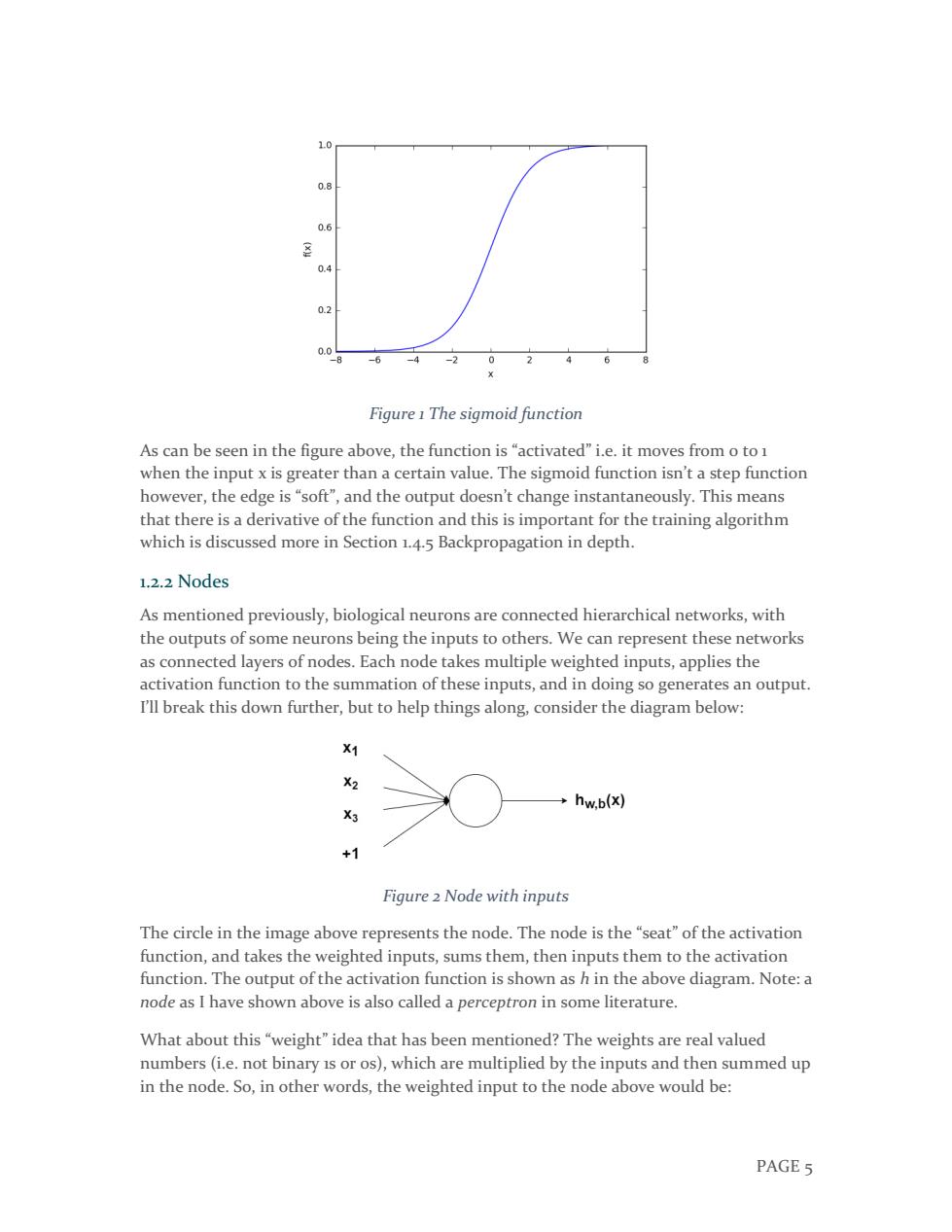
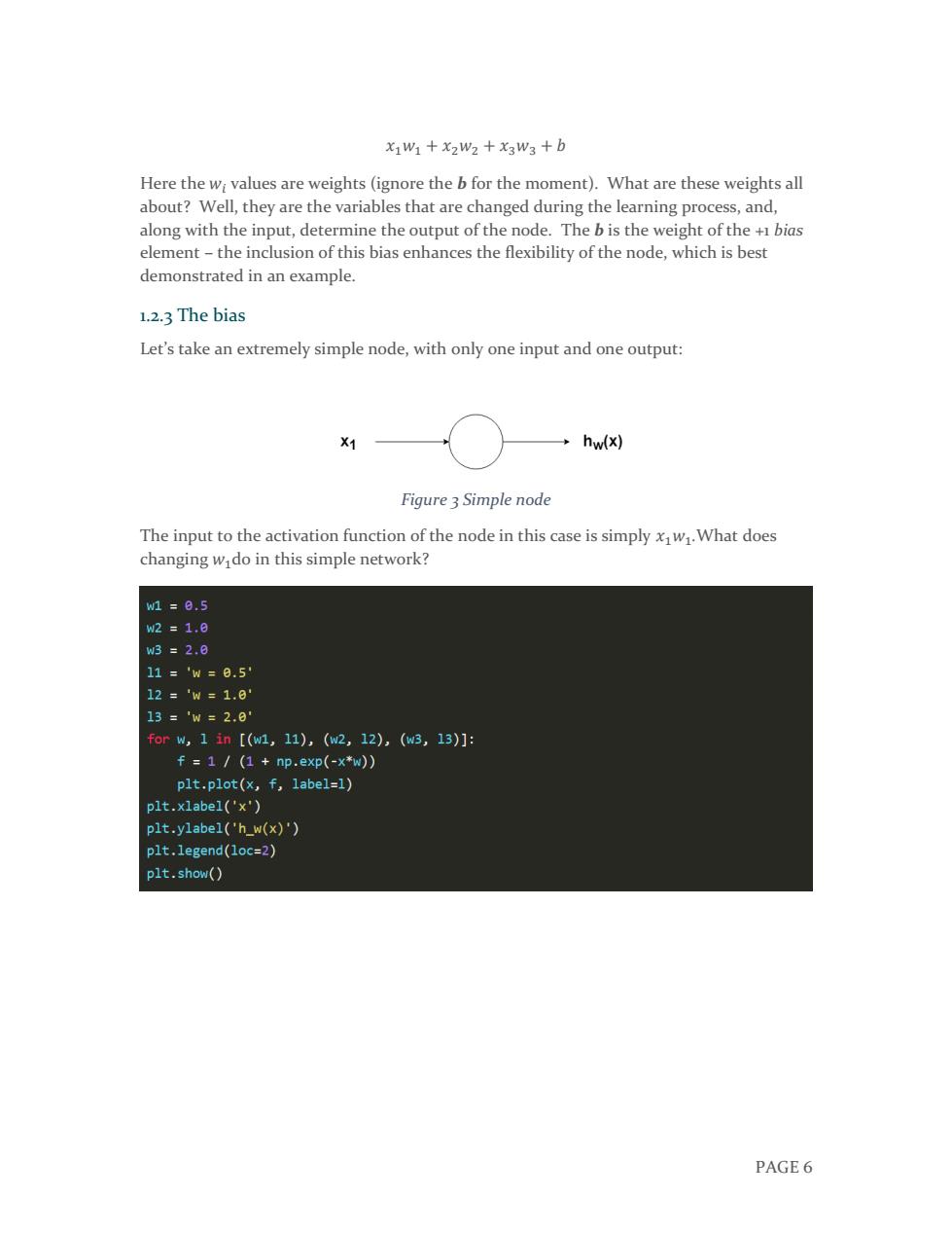
PAGE 5 Figure 1 The sigmoid function As can be seen in the figure above, the function is “activated” i.e. it moves from 0 to 1 when the input x is greater than a certain value. The sigmoid function isn’t a step function however, the edge is “soft”, and the output doesn’t change instantaneously. This means that there is a derivative of the function and this is important for the training algorithm which is discussed more in Section 1.4.5 Backpropagation in depth. 1.2.2 Nodes As mentioned previously, biological neurons are connected hierarchical networks, with the outputs of some neurons being the inputs to others. We can represent these networks as connected layers of nodes. Each node takes multiple weighted inputs, applies the activation function to the summation of these inputs, and in doing so generates an output. I’ll break this down further, but to help things along, consider the diagram below: Figure 2 Node with inputs The circle in the image above represents the node. The node is the “seat” of the activation function, and takes the weighted inputs, sums them, then inputs them to the activation function. The output of the activation function is shown as h in the above diagram. Note: a node as I have shown above is also called a perceptron in some literature. What about this “weight” idea that has been mentioned? The weights are real valued numbers (i.e. not binary 1s or 0s), which are multiplied by the inputs and then summed up in the node. So, in other words, the weighted input to the node above would be:
x1W1+x2W2+x3W3+b Here the wi values are weights(ignore the b for the moment).What are these weights all about?Well,they are the variables that are changed during the learning process,and, along with the input,determine the output of the node.The b is the weight of the +1 bias element-the inclusion of this bias enhances the flexibility of the node,which is best demonstrated in an example. 1.2.3 The bias Let's take an extremely simple node,with only one input and one output: X1 hw(x) Figure 3 Simple node The input to the activation function of the node in this case is simply xw.What does changing wi do in this simple network? w1=8.5 w2=1.8 w3=2.0 11='w=0.5 12='w=1.0 13='w=2.8 forw,1in[(w1,11),(w2,12),(w3,13)]: f=1/(1+np.exp(-x*w)) plt.plot(x,f,label=1) plt.xlabel('x') plt.ylabel('h_w(x)') plt.legend(loc=2) plt.show() PAGE6
PAGE 6 𝑥1𝑤1 + 𝑥2𝑤2 + 𝑥3𝑤3 + 𝑏 Here the 𝑤𝑖 values are weights (ignore the b for the moment). What are these weights all about? Well, they are the variables that are changed during the learning process, and, along with the input, determine the output of the node. The b is the weight of the +1 bias element – the inclusion of this bias enhances the flexibility of the node, which is best demonstrated in an example. 1.2.3 The bias Let’s take an extremely simple node, with only one input and one output: Figure 3 Simple node The input to the activation function of the node in this case is simply 𝑥1𝑤1.What does changing 𝑤1do in this simple network?
1.0 w=0.5 w=1.0 0.8 w=2.0 0.6 0.4 0.2 0.0 -6 -4 -2 0 2 6 Figure 4 Effect of adjusting weights Here we can see that changing the weight changes the slope of the output of the sigmoid activation function,which is obviously useful if we want to model different strengths of relationships between the input and output variables.However,what if we only want the output to change when x is greater than 1?This is where the bias comes in-let's consider the same network with a bias input: X1 W1 hw.b(x) 1 Figure 5 Node with bias PAGE 7
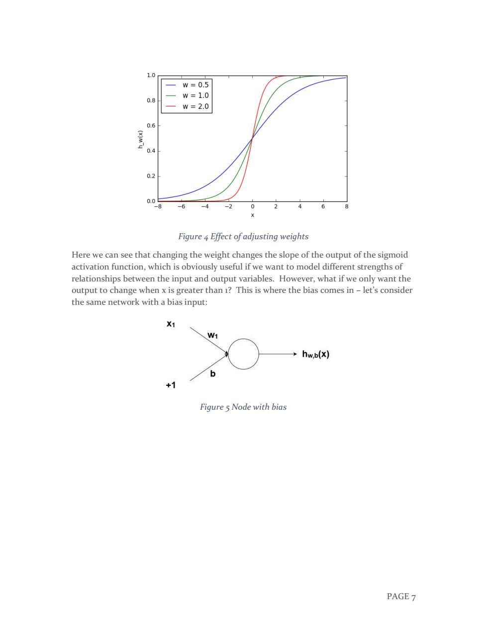
PAGE 7 Figure 4 Effect of adjusting weights Here we can see that changing the weight changes the slope of the output of the sigmoid activation function, which is obviously useful if we want to model different strengths of relationships between the input and output variables. However, what if we only want the output to change when x is greater than 1? This is where the bias comes in – let’s consider the same network with a bias input: Figure 5 Node with bias
w=5.8 b1=-8.0 b2=8.a b3=8.0 11=b=-8.8 12='b=6.8 13=b=8.0' forb,1in[(b1,11),(b2,12),(b3,13)]: f=1/(1+np.exp(-(x*w+b)) plt.plot(x,f,label=1) plt.xlabel('x') plt.ylabel('h_wb(x)') plt.legend(loc=2) plt.show() 1.0 b=-8.0 0.8 b=0.0 b=8.0 0.6 0.2 0.0 8 -6 -4 -20 2 6 8 Figure 6 Effect of bias adjustments In this case,the wi has been increased to simulate a more defined "turn on"function.As you can see,by varying the bias "weight"b,you can change when the node activates.Therefore,by adding a bias term,you can make the node simulate a generic if function,i.e.if(x>z)then 1 else o.Without a bias term,you are unable to vary the z in that if statement,it will be always stuck around o.This is obviously very useful if you are trying to simulate conditional relationships. 1.2.4 Putting together the structure Hopefully the previous explanations have given you a good overview of how a given node/neuron/perceptron in a neural network operates.However,as you are probably aware,there are many such interconnected nodes in a fully fledged neural network.These structures can come in a myriad of different forms,but the most common simple neural PAGE 8
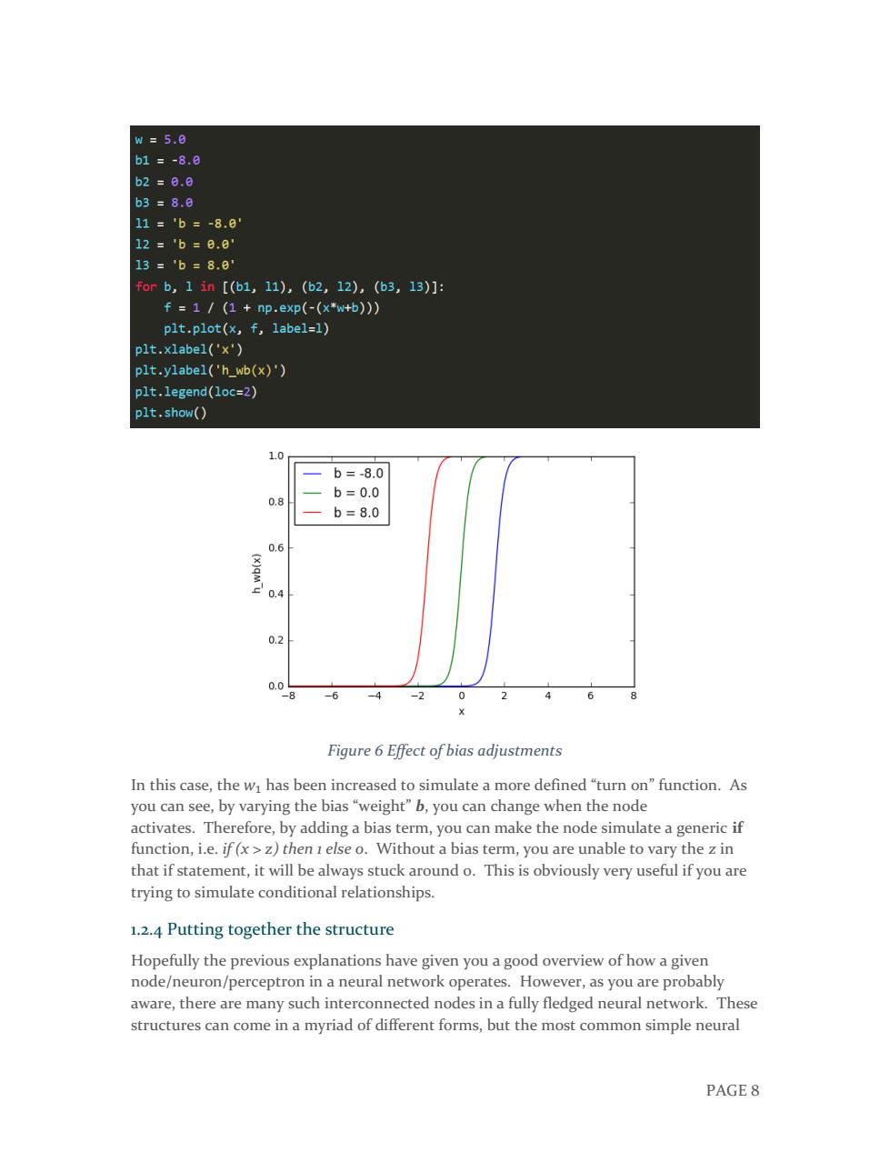
PAGE 8 Figure 6 Effect of bias adjustments In this case, the 𝑤1 has been increased to simulate a more defined “turn on” function. As you can see, by varying the bias “weight” b, you can change when the node activates. Therefore, by adding a bias term, you can make the node simulate a generic if function, i.e. if (x > z) then 1 else 0. Without a bias term, you are unable to vary the z in that if statement, it will be always stuck around 0. This is obviously very useful if you are trying to simulate conditional relationships. 1.2.4 Putting together the structure Hopefully the previous explanations have given you a good overview of how a given node/neuron/perceptron in a neural network operates. However, as you are probably aware, there are many such interconnected nodes in a fully fledged neural network. These structures can come in a myriad of different forms, but the most common simple neural
network structure consists of an input layer,a hidden layer and an output layer.An example of such a structure can be seen below: h,②) X X2 h22 h,3) hw.b(x) ha) Layer 1 Layer 2 Layer3 Figure 7 Three layer neural network The three layers of the network can be seen in the above figure-Layer 1 represents the input layer,where the external input data enters the network.Layer 2 is called the hidden layer as this layer is not part of the input or output.Note:neural networks can have many hidden layers,but in this case for simplicity I have just included one.Finally, Layer 3 is the output layer.You can observe the many connections between the layers,in particular between Layer 1(Li)and Layer 2(L2).As can be seen,each node in Li has a connection to all the nodes in L2.Likewise for the nodes in L2 to the single output node L3.Each of these connections will have an associated weight. 1.2.5 The notation The maths below requires some fairly precise notation so that we know what we are talking about.The notation I am using here is similar to that used in the Stanford deep learning tutorial.In the upcoming equations,each of these weights are identified with the following notation:wij.irefers to the node number of the connection in layer+1and j refers to the node number of the connection in layer I.Take special note of this order.So, for the connection between node 1 in layer 1 and node 2 in layer 2,the weight notation would be w21(1).This notation may seem a bit odd,as you would expect the i and jto refer the node numbers in layers I and l+1 respectively(i.e.in the direction of input to output),rather than the opposite.However,this notation makes more sense when you add the bias. As you can observe in the figure above-the (+1)bias is connected to each of the nodes in the subsequent layer.The bias in layer 1 is connected to the all the nodes in layer two. Because the bias is not a true node with an activation function,it has no inputs(it always outputs the value+).The notation of the bias weight is b,whereiis the node number in the layerl+1-the same as used for the normal weight notation w2().So,the PAGE 9
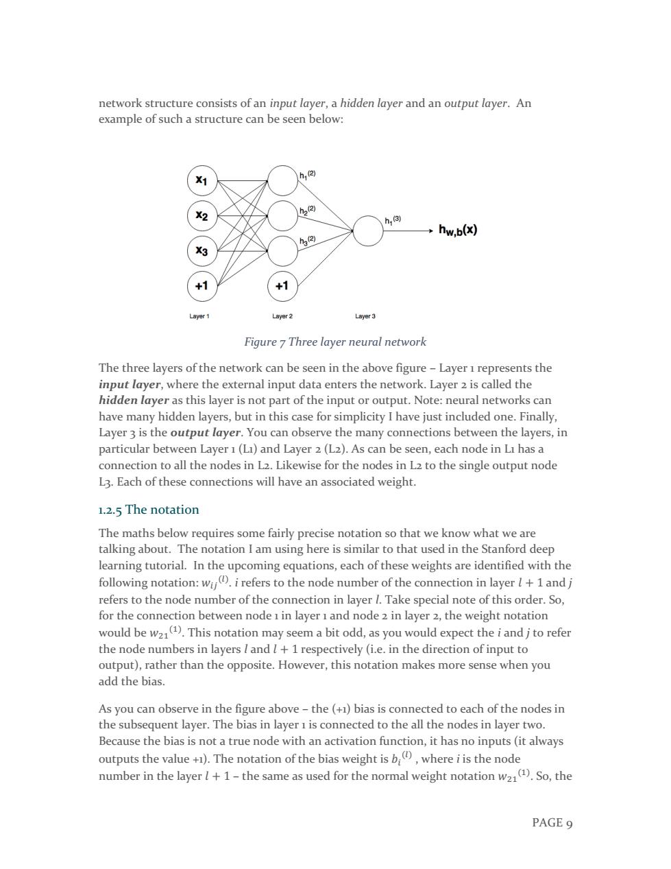
PAGE 9 network structure consists of an input layer, a hidden layer and an output layer. An example of such a structure can be seen below: Figure 7 Three layer neural network The three layers of the network can be seen in the above figure – Layer 1 represents the input layer, where the external input data enters the network. Layer 2 is called the hidden layer as this layer is not part of the input or output. Note: neural networks can have many hidden layers, but in this case for simplicity I have just included one. Finally, Layer 3 is the output layer. You can observe the many connections between the layers, in particular between Layer 1 (L1) and Layer 2 (L2). As can be seen, each node in L1 has a connection to all the nodes in L2. Likewise for the nodes in L2 to the single output node L3. Each of these connections will have an associated weight. 1.2.5 The notation The maths below requires some fairly precise notation so that we know what we are talking about. The notation I am using here is similar to that used in the Stanford deep learning tutorial. In the upcoming equations, each of these weights are identified with the following notation: 𝑤𝑖𝑗 (𝑙) . i refers to the node number of the connection in layer 𝑙 + 1 and j refers to the node number of the connection in layer l. Take special note of this order. So, for the connection between node 1 in layer 1 and node 2 in layer 2, the weight notation would be 𝑤21 (1) . This notation may seem a bit odd, as you would expect the i and j to refer the node numbers in layers l and 𝑙 + 1 respectively (i.e. in the direction of input to output), rather than the opposite. However, this notation makes more sense when you add the bias. As you can observe in the figure above – the (+1) bias is connected to each of the nodes in the subsequent layer. The bias in layer 1 is connected to the all the nodes in layer two. Because the bias is not a true node with an activation function, it has no inputs (it always outputs the value +1). The notation of the bias weight is 𝑏𝑖 (𝑙) , where i is the node number in the layer 𝑙 + 1 – the same as used for the normal weight notation 𝑤21 (1) . So, the