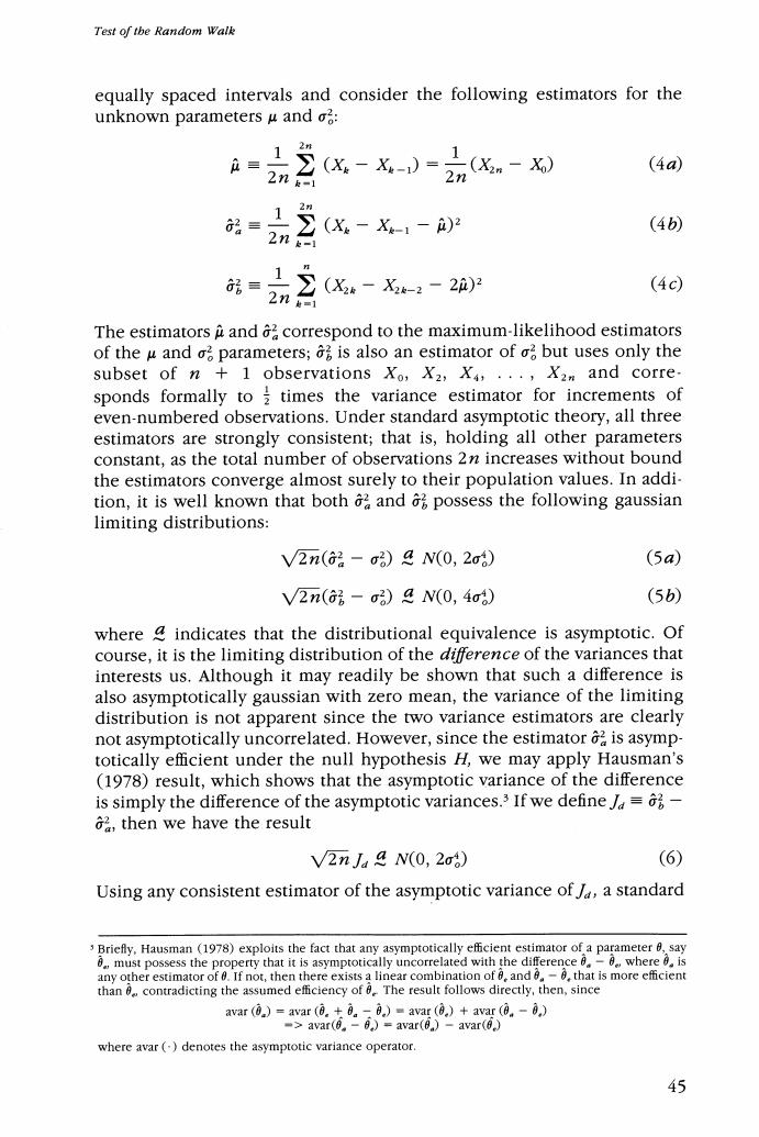
Test of tbe Random Walk equally spaced intervals and consider the following estimators for the unknown parameters u and o: 1 2排 (X。-X-)= 1(X2 -X) (4a) 2ne-1 2 品= 2 (4b) 2nk-1 (X。-X-1-)2 2(&-,-2 (4c) 2n0=1 The estimators a and correspond to the maximum-likelihood estimators of the u and o parameters;is also an estimator of o but uses only the subset of n 1 observations Xo,X2,X,...,X2m and corre. sponds formally to times the variance estimator for increments of even-numbered observations.Under standard asymptotic theory,all three estimators are strongly consistent;that is,holding all other parameters constant,as the total number of observations 2n increases without bound the estimators converge almost surely to their population values.In addi- tion,it is well known that both and possess the following gaussian limiting distributions: V2n(2-σ)4N(0,2o) (5a) V2n(3-o)&N(0,4o) (5b) where indicates that the distributional equivalence is asymptotic.Of course,it is the limiting distribution of the difference of the variances that interests us.Although it may readily be shown that such a difference is also asymptotically gaussian with zero mean,the variance of the limiting distribution is not apparent since the two variance estimators are clearly not asymptotically uncorrelated.However,since the estimator is asymp- totically efficient under the null hypothesis H,we may apply Hausman's (1978)result,which shows that the asymptotic variance of the difference is simply the difference of the asymptotic variances.3 If we define=- then we have the result V2n Ja 4 N(0,200) (6) Using any consistent estimator of the asymptotic variance of /a standard Briefy,Hausman (1978)exploits the fact that any asymptotically efficient estimator of a parameter 0,say 8.,must possess the property that it is asymptotically uncorrelated with the difference .-0.where 8.is any other estimator of 0.If not,then there exists a linear combination of and .-8,that is more efficient than 8,contradicting the assumed efficiency of 6.The result follows directly,then,since avar (0)avar (0.0.)=avar (0.)+avar (0-0) -avar(6.-6)=avar()-avar(6.) where avar (denotes the asymptotic variance operator. 45

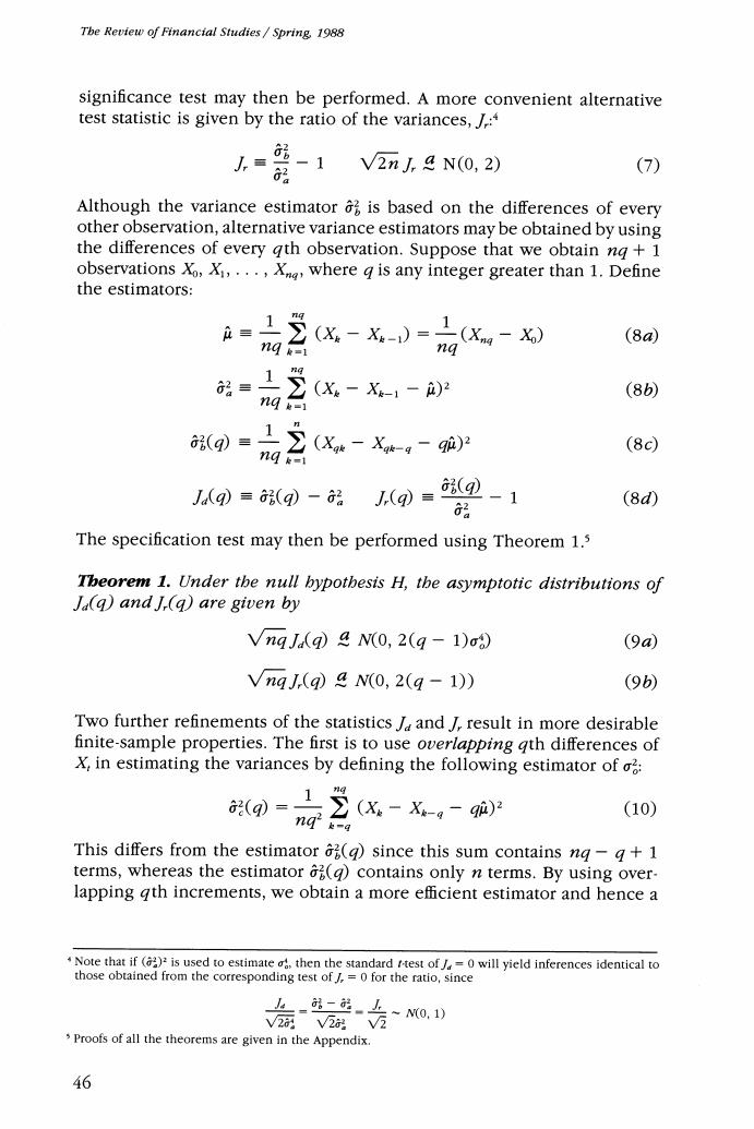
Tbe Review of Financial Studies/Spring,1988 significance test may then be performed.A more convenient alternative test statistic is given by the ratio of the variances,/: 人=-1 2 V2n,4N(0,2) (7) Although the variance estimator is based on the differences of every other observation,alternative variance estimators may be obtained by using the differences of every gth observation.Suppose that we obtain ng +1 observations X,Xi,...,X,where g is any integer greater than 1.Define the estimators: = x-X-)=(x-x (8a 1n☑e= ng 2(x-X&1- (8b) ng (g=22 (Xe-Xk-g-9驴)2 (8c) ng J(q)≡(q)-品 J(g)= 6(①-1 (8d) G经 The specification test may then be performed using Theorem 1.5 Tbeorem 1.Under the null bypotbesis H,the asymptotic distributions of la(q)andI(q)are given by VnqJaq)4 N(0,2(q-1)00) (9a VngJ(q)a N(0,2(g-1)) (9b Two further refinements of the statistics J and /result in more desirable finite-sample properties.The first is to use overlapping qth differences of X,in estimating the variances by defining the following estimator of 2(X-X-,-9m2 (10) This differs from the estimator (g)since this sum contains nq-g+1 terms,whereas the estimator (g)contains only n terms.By using over- lapping gth increments,we obtain a more efficient estimator and hence a Note that if ()is used to estimate,then the standard t-test of=0 will yield inferences identical to those obtained from the corresponding test of/,=0 for the ratio,since 上-i--5~N0,1) V2V2V2 Proofs of all the theorems are given in the Appendix. 46

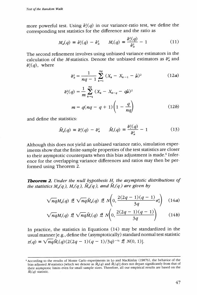
Test of the Random Walk more powerful test.Using 2()in our variance-ratio test,we define the corresponding test statistics for the difference and the ratio as M(q)=2(q)-2M,(q)= (①-1 (11) 62 The second refinement involves using unbiased variance estimators in the calculation of the M-statistics.Denote the unbiased estimators as and (g),where ng-1 觉(X-X-,- (12a) g=1(x-X-,- m m=q(ng- - (12b) and define the statistics: MAq)=(q)- a.()= (①-1 (13) G品 Although this does not yield an unbiased variance ratio,simulation exper- iments show that the finite-sample properties of the test statistics are closer to their asymptotic counterparts when this bias adjustment is made.s Infer- ence for the overlapping variance differences and ratios may then be per- formed using Theorem 2. Tbeorem 2.Under the null bypotbesis H,the asymptotic distributions of the statistics Ma(q),M,(q),Ma(q),and M.(q)are given by VngMa(q)a VngMd(g)4 N0, (29-1)(9-1) (14a 3q VnaM.o Vngn(No,22-D(g-1 (14b) 3q In practice,the statistics in Equations (14)may be standardized in the usual manner [e.g.,define the (asymptotically)standard normal test statistic z(q)=VngM,(q(2(2q-1)(q-1)/3q-N(0,1]: .According to the results of Monte Carlo experiments in Lo and Mackinlay (1987b),the behavior of the bias-adjusted M-statistics [which we denote as M()and M,()]does not depart significantly from that of their asymptotic limits even for small sample sizes.Therefore,all our empirical results are based on the M(g)statistic. 47

The Review of Financial Studies/Spring,1988 To develop some intuition for these variance ratios,observe that for an aggregation value g of 2,the M,()statistic may be reexpressed as 1 M2)=1)-4iaX-X-2+(x.-X-1-2月≥(10(15) Hence,for g=2 the M(g)statistic is approximately the first-order auto- correlation coefficient estimator p(1)of the differences.More generally,it may be shown that M(g)-29-卫1)+2g-262)+…+2(g-1) 2 (16) q q where (k)denotes the kth-order autocorrelation coefficient estimator of the first differences of X.7 Equation (16)provides a simple interpretation for the variance ratios computed with an aggregation value g:They are (approximately)linear combinations of the first g-1 autocorrelation coefficient estimators of the first differences with arithmetically declining weights.8 1.2 Heteroscedastic increments Since there is already a growing consensus among financial economists that volatilities do change over time,?a rejection of the random walk hypothesis because of heteroscedasticity would not be of much interest. We therefore wish to derive a version of our specification test of the random walk model that is robust to changing variances.As long as the increments are uncorrelated,even in the presence of heteroscedasticity the variance ratio must still approach unity as the number of observations increase without bound,for the variance of the sum of uncorrelated increments must still equal the sum of the variances.However,the asymptotic variance of the variance ratios will clearly depend on the type and degree of het- eroscedasticity present.One possible approach is to assume some specific form of heteroscedasticity and then to calculate the asymptotic variance of M,(g)under this null hypothesis.However,to allow for more general forms of heteroscedasticity,we employ an approach developed by White (1980)and by White and Domowitz (1984).This approach also allows us to relax the requirement of gaussian increments,an especially important See Equation (A2-2)in the Appendix. Note the similarity between these variance ratios and the Box-Pierce O-statistic,which is a linear combi- nation of squared autocorrelations with all the weights set identically equal to unity.Although we may expect the finite-sample behavior of the variance ratios to be comparable to that of the o-statistic under the null hypothesis,they can have very different power properties under various alternatives.See Lo and MacKinlay (1987b)for further details. See,for example,Merton (1980),Poterba and Summers (1986),and French,Schwert,and Stambaugh (1987). 48